Language Reference

EIGEN Call

CALL EIGEN (evals, evecs, A<VECL=vl>);

The EIGEN subroutine computes eigenvalues and eigenvectors of an arbitrary square numeric matrix. In SAS/IML 14.1 the EIGEN subroutine will use vendor-supplied eigenvalue routines if they are available on your system. (An example is the Intel Math Kernel Library (MKL), which is tuned to provide optimal performance for a given Intel processor.) Because eigenvectors are not unique, the results of eigenvector computations in SAS/IML 14.1 are not necessarily identical to the results from earlier releases. If you want to restore the pre-14.1 algorithm you can use the RESET EIGEN93 statement.

The A argument is the input argument to the EIGEN subroutine. The EIGEN call returns the following values:

evals: names a matrix to contain the eigenvalues of A.
evecs: names a matrix to contain the right eigenvectors of A.
vl: is an optional $n \times n$ matrix that contains the left eigenvectors of A in the same manner that evecs contains the right eigenvectors.

The EIGEN subroutine computes evals, a matrix that contains the eigenvalues of A. If A is symmetric, evals is the $n \times 1$ vector that contains the n real eigenvalues of A. If A is not symmetric (as determined by the criteria in the symmetry test described later), evals is an $n \times 2$ matrix. The first column of evals contains the real parts, $\mbox{Re}(\lambda )$ , and the second column contains the imaginary parts, $\mbox{Im}(\lambda )$ . Each row represents one eigenvalue, $\mbox{Re}(\lambda ) + i\mbox{Im}(\lambda )$ .

If A is symmetric, the eigenvalues are arranged in descending order. Otherwise, the eigenvalues are sorted first by their real parts, then by the magnitude of their imaginary parts. Complex conjugate eigenvalues, $\mbox{Re}(\lambda )\pm i\mbox{Im}(\lambda )$ , are stored in standard order; that is, the eigenvalue of the pair with a positive imaginary part is followed by the eigenvalue of the pair with the negative imaginary part.

The EIGEN subroutine also computes evecs, a matrix that contains the orthonormal column eigenvectors that correspond to evals. If A is symmetric, then the first column of evecs is the eigenvector that corresponds to the largest eigenvalue, and so forth. If A is not symmetric, then evecs is an $n \times n$ matrix that contains the right eigenvectors of A. If the eigenvalue in row i of evals is real, then column i of evecs contains the corresponding real eigenvector. If rows i and $i+1$ of evals contain complex conjugate eigenvalues $\mbox{Re}(\lambda )\pm i\mbox{Im}(\lambda )$ , then columns i and $i+1$ of evecs contain the real part, $\mb{u}$ , and imaginary part, $\mb{v}$ , of the two corresponding eigenvectors $\mb{u}\pm i\mb{v}$ .

The following paragraphs present some properties of eigenvalues and eigenvectors. Let $\bA$ be a general $n\times n$ matrix. The eigenvalues of $\bA$ are the roots of the characteristic polynomial, which is defined as $p(z) = \det (z\bI - \bA )$ . The spectrum, denoted by $\lambda (A)$ , is the set of eigenvalues of the matrix A. If $\lambda (\bA )=\{ \lambda _1,\ldots ,\lambda _ n\}$ , then $\det (\bA ) = \lambda _1 \lambda _2 \cdots \lambda _ n$ .

The trace of $\bA$ is defined by

$\mr{tr}(\bA ) = \sum _{i=1}^ n a_{ii}$

and tr $(\bA )= \lambda _1 + \ldots + \lambda _ n$ .

An eigenvector is a nonzero vector, $\mb{x}$ , that satisfies $\bA \mb{x} = \lambda \mb{x}$ for $\lambda \in \lambda (\bA )$ . Right eigenvectors satisfy $\bA \mb{x} = \lambda \mb{x}$ , and left eigenvectors satisfy $\mb{x}^{H}\bA = \lambda \mb{x}^{H}$ , where $\mb{x}^{H}$ is the complex conjugate transpose of $\mb{x}$ . Taking the conjugate transpose of both sides shows that left eigenvectors also satisfy $\bA ^{\prime }\mb{x} = \bar{\lambda }\mb{x}$ .

The following are properties of the unsymmetric real eigenvalue problem, in which the real matrix $\bA$ is square but not necessarily symmetric:

The eigenvalues of an unsymmetric matrix $\bA$ can be complex. If $\bA$ has a complex eigenvalue, $\mbox{Re}(\lambda )+i\mbox{Im}(\lambda )$ , then the conjugate complex value $\mbox{Re}(\lambda )-i\mbox{Im}(\lambda )$ is also an eigenvalue of $\bA$ .
The right and left eigenvectors that correspond to a real eigenvalue of $\bA$ are real. The right and left eigenvectors that correspond to conjugate complex eigenvalues of $\bA$ are also conjugate complex.
The left eigenvectors of $\bA$ are the same as the complex conjugate right eigenvectors of $\bA ^{\prime }$ .

The three routines, EIGEN, EIGVAL, and EIGVEC, use the following test of symmetry for a square argument matrix $\bA$ :

Select the entry of $\bA$ with the largest magnitude:

$a_{max} = \max _{i,j=1,\ldots ,n} |a_{i,j}|$
Multiply the value of $a_{max}$ by the square root of the machine precision, $\epsilon$ . The value of $\epsilon$ is the largest value stored in double precision that, when added to 1 in double precision, still results in 1.
The matrix $\bA$ is considered unsymmetric if there exists at least one pair of symmetric entries that differs in more than $a_{max}\sqrt {\epsilon }$ :

$|a_{i,j}-a_{j,i}| > a_{max} \sqrt {\epsilon }$

If $\bA$ is a symmetric matrix and $\bM$ and $\bE$ are the eigenvalues and eigenvectors, respectively, of $\bA$ , then the matrices have the following properties:

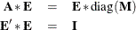
$\begin{eqnarray*} \bA *\bE & = & \bE *\mbox{diag}(\bM ) \\ \bE ^{\prime }*\bE & = & \bI \end{eqnarray*}$

These properties imply the following:

$\bE ^{\prime } = \mbox{inv}(\bE )$

$\bA = \bE *\mbox{diag}(\bM )*\bE ^{\prime }$

The QL method is used to compute the eigenvalues (Wilkinson and Reinsch 1971).

In statistical applications, nonsymmetric matrices for which eigenvalues are desired are usually of the form $\bE ^{-1} \mb{H}$ , where $\bE$ and $\mb{H}$ are symmetric. The eigenvalues $\mb{L}$ and eigenvectors $\bV$ of $\bE ^{-1}\mb{H}$ can be obtained by using the GENEIG subroutine , or by using the following statements:

F = root(einv);
A = F*H*F`;
call eigen(L, W, A);
V = F`*W;

The computation can be checked by forming the residuals, r, as shown in the following statement:

r = einv*H*V - V*diag(L);

The values in r should be of the order of rounding error.

The following statements compute the eigenvalues and left and right eigenvectors of a nonsymmetric matrix with four real and four complex eigenvalues:

A = {-1  2  0       0       0       0       0  0,
     -2 -1  0       0       0       0       0  0,
      0  0  0.2379  0.5145  0.1201  0.1275  0  0,
      0  0  0.1943  0.4954  0.1230  0.1873  0  0,
      0  0  0.1827  0.4955  0.1350  0.1868  0  0,
      0  0  0.1084  0.4218  0.1045  0.3653  0  0,
      0  0  0       0       0       0       2  2,
      0  0  0       0       0       0      -2  0 };
call eigen(val, rvec, A) vecl="lvec";
print val;

The sorted eigenvalues of the A matrix are shown in Figure 25.117.

Figure 25.117: Complex Eigenvalues of a Nonsymmetric Matrix

val
1	1.7320508
1	-1.732051
1	0
0.2087788	0
0.0222025	0
0.0026187	0
-1	2
-1	-2

You can verify the correctness of the left and right eigenvector computation by using the following statements:

/* verify that the right eigenvectors are correct */
vec = rvec;
do j = 1 to ncol(vec);
  /* if eigenvalue is real */
  if val[j,2] = 0. then do;
    v = A * vec[,j] - val[j,1] * vec[,j];
    if any( abs(v) > 1e-12 ) then
      badVectors = badVectors || j;
    end;
  /* if eigenvalue is complex with positive imaginary part */
  else if val[j,2] > 0. then do;
    /* the real part */
    rp = val[j,1] * vec[,j] - val[j,2] * vec[,j+1];
    v = A * vec[,j] - rp;
    /* the imaginary part */
    ip = val[j,1] * vec[,j+1] + val[j,2] * vec[,j];
    u = A * vec[,j+1] - ip;
    if any( abs(u) > 1e-12 ) | any( abs(v) > 1e-12 ) then
      badVectors = badVectors || j || j+1;
    end;
  end;
if ncol( badVectors ) > 0 then
  print "Incorrect right eigenvectors:" badVectors;
else print "All right eigenvectors are correct";

Similar statements can be written to verify the left eigenvectors. The statements use the fact that the left eigenvectors of $\bA$ are the same as the complex conjugate right eigenvectors of $\bA ^{\prime }$ :

/* verify that the left eigenvectors are correct */
vec = lvec;
do j = 1 to ncol(vec);
  /* if eigenvalue is real */
  if val[j,2] = 0. then do;
    v = A` * vec[,j] - val[j,1] * vec[,j];
    if any( abs(v) > 1e-12 ) then
      badVectors = badVectors || j;
    end;
  /* if eigenvalue is complex with positive imaginary part */
  else if val[j,2] > 0. then do;
    /* Note the use of complex conjugation */
    /* the real part */
    rp = val[j,1] * vec[,j] + val[j,2] * vec[,j+1];
    v = A` * vec[,j] - rp;
    /* the imaginary part */
    ip = val[j,1] * vec[,j+1] - val[j,2] * vec[,j];
    u = A` * vec[,j+1] - ip;
    if any( abs(u) > 1e-12 ) | any( abs(v) > 1e-12 ) then
      badVectors = badVectors || j || j+1;
    end;
  end;
if ncol( badVectors ) > 0 then
  print "Incorrect left eigenvectors:" badVectors;
else print "All left eigenvectors are correct";

The EIGEN call performs most of its computations in the memory allocated for returning the eigenvectors.