General Statistics Examples
Example 10.8 Logistic and Probit Regression for Binary Response Models
A binary response Y is fit to a linear model according to
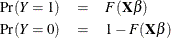
where F is some smooth probability distribution function. In this example, the normal and logistic distributions are used.
The regression computes parameter estimates by using maximum likelihood via iteratively reweighted least squares, as described
in Charnes, Frome, and Yu (1976); Jennrich and Moore (1975); Nelder and Wedderburn (1972). Rows are scaled by the derivative of the distribution, which is the density. The weights are assigned by using the expression
 , where w is a count or some other weight.
The following statements define the module BINEST, which computes logistic and probit regressions for binary response models:
proc iml ;
/* compute density function (PDF) */
start Density(model, z);
   if upcase(model)='LOGIT'  then
      return( pdf("Logistic", z) );
   else /* "PROBIT" */
      return( pdf("Normal", z) );
finish;

/* compute cumulative distribution function (CDF) */
start Distrib(model, z);
   if upcase(model)='LOGIT'  then
      return( cdf("Logistic", z) );
   else /* "PROBIT" */
      return( cdf("Normal", z) );
finish;

/* routine for estimating binary response models             */
/* model is "logit" or "probit"                              */
/* varNames has the names of the regressor variables         */
start BinEst(nEvents, nTrials, data, model, varNames);
   /* set up design matrix */
   n = nrow(data);
   x = j(n,1,1) || data;                       /* add intercept */
   x = x // x;                                    /* regressors */
   y = j(n,1,1) // j(n,1,0);      /* binary response: 1s and 0s */
   wgt = nEvents // (nTrials-nEvents);         /* count weights */

   parms = "Intercept" || rowvec(varNames);
   k = ncol(x);
   b = j(k,1,0);                             /* starting values */
   oldb = b+1;
   results = j(20, 2+k, .);          /* store iteration history */
   do iter=1 to nrow(results) while(max(abs(b-oldb))>1e-8);
      oldb = b;
      z = x*b;
      p = Distrib(model, z);
      loglik = sum( wgt#((y=1)#log(p) + (y=0)#log(1-p)) );
      results[iter, ] = iter || loglik || b`;
      w = wgt / (p#(1-p));
      f = Density(model, z);
      xx = f#x;
      xpxi = inv(xx`*(w#xx));
      b = b + xpxi*(xx`*(w#(y-p)));
   end;
   idx = loc(results^=.);    /* trim results if few iterations */
   results = shape(results[idx],0,2+ncol(parms));
   colnames = {"Iter" "LogLik"} || parms;
   lbl = "Iteration History: " + model + " Model";
   print results[colname=colnames label=lbl];

   p0 = sum((y=1)#wgt) / sum(wgt);           /* average response */
   loglik0 = sum( wgt#((y=1)#log(p0) + (y=0)#log(1-p0)) );
   chisq = 2#(loglik-loglik0);
   df = k-1;
   prob = 1 - cdf("ChiSq", chisq, df);
   stats = chisq || df || prob;
   print stats[colname={'ChiSq' 'DF' 'Prob'}
               label='Likelihood Ratio, Intercept-only Model'];

   stderr = sqrt(vecdiag(xpxi));
   tRatio = b/stderr;
   print (parms`)[label="parms"] b stderr tRatio;
finish;
The following statements call the BINEST module to compute a logistic regression for data that appear in Cox and Snell (1989, pp. 10–11). The data consist of the number of ingots that are not ready for rolling (nReady) and the total number tested (nTested) for a number of combinations of heating time and soaking time. The results are shown in Output 10.8.1.
data={ 7 1.0 0 10, 14 1.0 0 31, 27 1.0 1 56, 51 1.0 3 13,
       7 1.7 0 17, 14 1.7 0 43, 27 1.7 4 44, 51 1.7 0  1,
       7 2.2 0  7, 14 2.2 2 33, 27 2.2 0 21, 51 2.2 0  1,
       7 2.8 0 12, 14 2.8 0 31, 27 2.8 1 22,
       7 4.0 0  9, 14 4.0 0 19, 27 4.0 1 16, 51 4.0 0  1};
x = data[, 1:2];
parms = {"Heat" "Soak"};
nReady = data[, 3];
nTotal = data[, 4];

run BinEst(nReady, nTotal, x, "Logit", parms);     /* run logit model  */
Output 10.8.1: Logistic Regression: Results
| Iteration History: Logit Model | ||||
|---|---|---|---|---|
| Iter | LogLik | Intercept | Heat | Soak |
| 1 | -268.248 | 0 | 0 | 0 |
| 2 | -76.29481 | -2.159406 | 0.0138784 | 0.0037327 |
| 3 | -53.38033 | -3.53344 | 0.0363154 | 0.0119734 |
| 4 | -48.34609 | -4.748899 | 0.0640013 | 0.0299201 |
| 5 | -47.69191 | -5.413817 | 0.0790272 | 0.04982 |
| 6 | -47.67283 | -5.553931 | 0.0819276 | 0.0564395 |
| 7 | -47.67281 | -5.55916 | 0.0820307 | 0.0567708 |
| 8 | -47.67281 | -5.559166 | 0.0820308 | 0.0567713 |
You can use the LOGISTIC procedure in SAS/STAT software to perform a similar analysis. See the section "Getting Started: Logistic Procedure" in SAS/STAT User's Guide.
In a similar way, you can call the BINEST module and request a probit-model regression. The results, which appear in Output 10.8.2, are consistent with results from the PROBIT procedure.
run BinEst(nReady, nTotal, x, "Probit", parms); /* run probit model */
Output 10.8.2: Probit Regression: Results
| Iteration History: Logit Model | ||||
|---|---|---|---|---|
| Iter | LogLik | Intercept | Heat | Soak |
| 1 | -268.248 | 0 | 0 | 0 |
| 2 | -76.29481 | -2.159406 | 0.0138784 | 0.0037327 |
| 3 | -53.38033 | -3.53344 | 0.0363154 | 0.0119734 |
| 4 | -48.34609 | -4.748899 | 0.0640013 | 0.0299201 |
| 5 | -47.69191 | -5.413817 | 0.0790272 | 0.04982 |
| 6 | -47.67283 | -5.553931 | 0.0819276 | 0.0564395 |
| 7 | -47.67281 | -5.55916 | 0.0820307 | 0.0567708 |
| 8 | -47.67281 | -5.559166 | 0.0820308 | 0.0567713 |