Nonlinear Optimization Examples
The input argument tc specifies a vector of bounds that correspond to a set of termination criteria that are tested in each iteration. If you do not specify an IML module with the "ptit" argument, these bounds determine when the optimization process stops.
If you specify the "ptit" argument, the "tc" argument is ignored. The module specified by the "ptit" argument replaces the subroutine that is used by default to test the termination criteria. The module is called in each iteration
with the current location, x, and the value, f, of the objective function at x. The module must give a return code, ![]() , that decides whether the optimization process is to be continued or terminated. As long as the module returns
, that decides whether the optimization process is to be continued or terminated. As long as the module returns ![]() , the optimization process continues. When the module returns
, the optimization process continues. When the module returns ![]() , the optimization process stops.
, the optimization process stops.
If you use the tc vector, the optimization techniques stop the iteration process when at least one of the corresponding set of termination criteria are satisfied. Table 14.3 and Table 14.4 indicate the criterion associated with each element of the tc vector. There is a default for each criterion, and if you specify a missing value for the corresponding element of the tc vector, the default value is used. You can avoid termination with respect to the ABSFTOL, ABSGTOL, ABSXTOL, FTOL, FTOL2, GTOL, GTOL2, and XTOL criteria by specifying a value of zero for the corresponding element of the tc vector.
Table 14.3: Termination Criteria for the NLPNMS Subroutine
|
Index |
Description |
|---|---|
|
1 |
maximum number of iterations (MAXIT) |
|
2 |
maximum number of function calls (MAXFU) |
|
3 |
absolute function criterion (ABSTOL) |
|
4 |
relative function criterion (FTOL) |
|
5 |
relative function criterion (FTOL2) |
|
6 |
absolute function criterion (ABSFTOL) |
|
7 |
FSIZE value used in FTOL criterion |
|
8 |
relative parameter criterion (XTOL) |
|
9 |
absolute parameter criterion (ABSXTOL) |
|
9 |
size of final trust-region radius |
|
10 |
XSIZE value used in XTOL criterion |
Table 14.4: Termination Criteria for Other Subroutines
|
Index |
Description |
|---|---|
|
1 |
maximum number of iterations (MAXIT) |
|
2 |
maximum number of function calls (MAXFU) |
|
3 |
absolute function criterion (ABSTOL) |
|
4 |
relative gradient criterion (GTOL) |
|
5 |
relative gradient criterion (GTOL2) |
|
6 |
absolute gradient criterion (ABSGTOL) |
|
7 |
relative function criterion (FTOL) |
|
8 |
predicted function reduction criterion (FTOL2) |
|
9 |
absolute function criterion (ABSFTOL) |
|
10 |
FSIZE value used in GTOL and FTOL criterion |
|
11 |
relative parameter criterion (XTOL) |
|
12 |
absolute parameter criterion (ABSXTOL) |
|
13 |
XSIZE value used in XTOL criterion |
The following list indicates the termination criteria that are used with all the optimization techniques:
-
tc[1] specifies the maximum number of iterations in the optimization process (MAXIT). The default values are
NLPNMS:
MAXIT=1000
NLPCG:
MAXIT=400
Others:
MAXIT=200
-
tc[2] specifies the maximum number of function calls in the optimization process (MAXFU). The default values are
NLPNMS:
MAXFU=3000
NLPCG:
MAXFU=1000
Others:
MAXFU=500
-
tc[3] specifies the absolute function convergence criterion (ABSTOL). For minimization, termination requires
 ABSTOL, while for maximization, termination requires
  ABSTOL. The default values are the negative and positive square roots of the largest double precision value, for minimization and
maximization, respectively.
ABSTOL. The default values are the negative and positive square roots of the largest double precision value, for minimization and
maximization, respectively.
These criteria are useful when you want to divide a time-consuming optimization problem into a series of smaller problems.
Since the Nelder-Mead simplex algorithm does not use derivatives, no termination criteria are available that are based on the gradient of the objective function.
When the NLPNMS subroutine implements Powell’s COBYLA algorithm, it uses only one criterion other than the three used by all
the optimization techniques. The COBYLA algorithm is a trust-region method that sequentially reduces the radius, ![]() , of a spheric trust region from the start radius,
, of a spheric trust region from the start radius, ![]() , which is controlled with the par[2] argument, to the final radius,
, which is controlled with the par[2] argument, to the final radius, ![]() , which is controlled with the tc[9] argument. The default value for tc[9] is
, which is controlled with the tc[9] argument. The default value for tc[9] is ![]() 1E–4. Convergence to small values of
1E–4. Convergence to small values of ![]() can take many calls of the function and constraint modules and might result in numerical problems.
can take many calls of the function and constraint modules and might result in numerical problems.
In addition to the criteria used by all techniques, the original Nelder-Mead simplex algorithm uses several other termination criteria, which are described in the following list:
-
tc[4] specifies the relative function convergence criterion (FTOL). Termination requires a small relative difference between the function values of the vertices in the simplex with the largest and smallest function values.
![\[ { | f_{hi}^{(k)} - f_{lo}^{(k)} | \over \max (|f_{hi}^{(k)})|, \mathit{FSIZE}) } \leq \mathit{FTOL} \]](images/imlug_nonlinearoptexpls0158.png)
where FSIZE is defined by tc[7]. The default value is tc
![$[4] = 10^{-{\scriptstyle \mbox{FDIGITS}}}$](images/imlug_nonlinearoptexpls0159.png) , where FDIGITS is controlled by the par[8] argument. The par[8] argument has a default value of
, where FDIGITS is controlled by the par[8] argument. The par[8] argument has a default value of  , where
  is the machine precision. Hence, the default value for FTOL is .
-
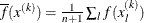
tc[5] specifies another relative function convergence criterion (FTOL2). Termination requires a small standard deviation of the function values of the
 simplex vertices
  .
.
![\[ \sqrt {{1 \over n+1} \sum _ l (f(x_ l^{(k)}) - \overline{f}(x^{(k)}))^2 } \leq \mathit{FTOL2} \]](images/imlug_nonlinearoptexpls0163.png)
where
 . If there are a active boundary constraints at
  , the mean and standard deviation are computed only for the
  unconstrained vertices. The default is tc
![$[5]=$](images/imlug_nonlinearoptexpls0166.png) 1E–6.
1E–6.
-
tc[6] specifies the absolute function convergence criterion (ABSFTOL). Termination requires a small absolute difference between the function values of the vertices in the simplex with the largest and smallest function values.
![\[ | f_{hi}^{(k)} - f_{lo}^{(k)} | \leq \mathit{ABSFTOL} \]](images/imlug_nonlinearoptexpls0167.png)
The default is tc
![$[6]=0$](images/imlug_nonlinearoptexpls0168.png) .
.
-
tc[7] specifies the FSIZE value used in the FTOL termination criterion. The default is tc
![$[7]=0$](images/imlug_nonlinearoptexpls0169.png) .
.
-
tc[8] specifies the relative parameter convergence criterion (XTOL). Termination requires a small relative parameter difference between the vertices with the largest and smallest function values.
![\[ {\max _ j |x_ j^{lo} - x_ j^{hi}| \over \max (|x_ j^{lo}|,|x_ j^{hi}|, \mathit{XSIZE})} \leq \mathit{XTOL} \]](images/imlug_nonlinearoptexpls0170.png)
The default is tc
![$[8]=$](images/imlug_nonlinearoptexpls0171.png) 1E–8.
1E–8.
-
tc[9] specifies the absolute parameter convergence criterion (ABSXTOL). Termination requires either a small length,
 , of the vertices of a restart simplex or a small simplex size,
  .
.
where
is defined as the L1 distance of the simplex vertex with the smallest function value,  , to the other n simplex points,
  .
.
![\[ \delta ^{(k)} = \sum _{x_ l \neq y} \parallel x_ l^{(k)} - y^{(k)} \parallel _1 \]](images/imlug_nonlinearoptexpls0177.png)
The default is tc
![$[9]=$](images/imlug_nonlinearoptexpls0178.png) 1E–8.
1E–8.
-
tc[10] specifies the XSIZE value used in the XTOL termination criterion. The default is tc
![$[10]=0$](images/imlug_nonlinearoptexpls0179.png) .
.
-
tc[4] specifies the relative gradient convergence criterion (GTOL). For all techniques except the NLPCG subroutine, termination requires that the normalized predicted function reduction is small.
![\[ { g(x^{(k)})^ T [G^{(k)}]^{-1} g(x^{(k)}) \over \max (|f(x^{(k)})|,\mathit{FSIZE}) } \leq \mathit{GTOL} \]](images/imlug_nonlinearoptexpls0180.png)
where FSIZE is defined by tc[10]. For the NLPCG technique (where a reliable Hessian estimate is not available),
![\[ { \parallel g(x^{(k)}) \parallel _2^2 \quad \parallel s(x^{(k)}) \parallel _2 \over \parallel g(x^{(k)}) - g(x^{(k-1)}) \parallel _2 \max (|f(x^{(k)})|, \mathit{FSIZE}) } \leq \mathit{GTOL} \]](images/imlug_nonlinearoptexpls0181.png)
is used. The default is tc
![$[4]=$](images/imlug_nonlinearoptexpls0182.png) 1E–8.
1E–8.
-
tc[5] specifies another relative gradient convergence criterion (GTOL2). This criterion is used only by the NLPLM subroutine.
![\[ \max _ j {|g_ j(x^{(k)})| \over \sqrt {f(x^{(k)}) G_{j,j}^{(k)}} } \leq \mathit{GTOL2} \]](images/imlug_nonlinearoptexpls0183.png)
The default is tc[5]=0.
-
tc[6] specifies the absolute gradient convergence criterion (ABSGTOL). Termination requires that the maximum absolute gradient element be small.
![\[ \max _ j |g_ j(x^{(k)})| \leq \mathit{ABSGTOL} \]](images/imlug_nonlinearoptexpls0184.png)
-
tc[7] specifies the relative function convergence criterion (FTOL). Termination requires a small relative change of the function value in consecutive iterations.
![\[ { |f(x^{(k)}) - f(x^{(k-1)})| \over \max (|f(x^{(k-1)})|,FSIZE) } \leq \mathit{FTOL} \]](images/imlug_nonlinearoptexpls0186.png)
where
 is defined by tc[10]. The default is tc
![$[7] = 10^{-{\scriptstyle \mbox{FDIGITS}}}$](images/imlug_nonlinearoptexpls0188.png) , where FDIGITS is controlled by the par[8] argument. The par[8] argument has a default value of , where is the machine precision. Hence, the default for FTOL is .
, where FDIGITS is controlled by the par[8] argument. The par[8] argument has a default value of , where is the machine precision. Hence, the default for FTOL is .
-
tc[8] specifies another function convergence criterion (FTOL2). For least squares problems, termination requires a small predicted reduction of the objective function,
 . The predicted reduction is computed by approximating the objective function by the first two terms of the Taylor series
and substituting the Newton step,
. The predicted reduction is computed by approximating the objective function by the first two terms of the Taylor series
and substituting the Newton step, 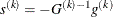 , as follows:
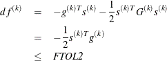
The FTOL2 criterion is the unscaled version of the GTOL criterion. The default is tc[8]=0.
-
tc[9] specifies the absolute function convergence criterion (ABSFTOL). Termination requires a small change of the function value in consecutive iterations.
![\[ |f(x^{(k-1)}) - f(x^{(k)})| \leq \mathit{ABSFTOL} \]](images/imlug_nonlinearoptexpls0192.png)
The default is tc[9]=0.
-
tc[10] specifies the FSIZE value used in the GTOL and FTOL termination criteria. The default is tc[10]=0.
-
tc[11] specifies the relative parameter convergence criterion (XTOL). Termination requires a small relative parameter change in consecutive iterations.
![\[ {\max _ j |x_ j^{(k)} - x_ j^{(k-1)}| \over \max (|x_ j^{(k)}|,|x_ j^{(k-1)}|,\mathit{XSIZE})} \leq \mathit{XTOL} \]](images/imlug_nonlinearoptexpls0193.png)
The default is tc[11]=0.
-
tc[12] specifies the absolute parameter convergence criterion (ABSXTOL). Termination requires a small Euclidean distance between parameter vectors in consecutive iterations.
![\[ \parallel x^{(k)} - x^{(k-1)} \parallel _2 \leq \mathit{ABSXTOL} \]](images/imlug_nonlinearoptexpls0194.png)
The default is tc[12]=0.
-
tc[13] specifies the XSIZE value used in the XTOL termination criterion. The default is tc[13]=0.
The only algorithm available for nonlinearly constrained optimization other than the NLPNMS subroutine is the NLPQN subroutine, when you specify the "nlc" module argument. This method, unlike the other optimization methods, does not monotonically reduce the value of the objective function or some kind of merit function that combines objective and constraint functions. Instead, the algorithm uses the watchdog technique with backtracking of Chamberlain et al. (1982). Therefore, no termination criteria are implemented that are based on the values x or f in consecutive iterations. In addition to the criteria used by all optimization techniques, there are three other termination criteria available; these are based on the Lagrange function
and its gradient
where m denotes the total number of constraints, ![]() is the gradient of the objective function, and
is the gradient of the objective function, and ![]() is the vector of Lagrange multipliers. The Kuhn-Tucker conditions require that the gradient of the Lagrange function is zero
at the optimal point
is the vector of Lagrange multipliers. The Kuhn-Tucker conditions require that the gradient of the Lagrange function is zero
at the optimal point ![]() , as follows:
, as follows:
-
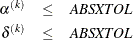
tc[4] specifies the GTOL criterion, which requires that the normalized predicted function reduction be small.
![\[ { { |g(x^{(k)}) s(x^{(k)})| + \sum _{i=1}^ m |\lambda _ i c_ i(x^{(k)})| } \over { \max (|f(x^{(k)})|, \mathit{FSIZE}) } } \leq \mathit{GTOL} \]](images/imlug_nonlinearoptexpls0200.png)
where FSIZE is defined by the tc[10] argument. The default is tc
1E–8.
-
tc[6] specifies the ABSGTOL criterion, which requires that the maximum absolute gradient element of the Lagrange function be small.
![\[ \max _ j | \{ \nabla _ x L(x^{(k)},\lambda ^{(k)})\} _ j | \leq \mathit{ABSGTOL} \]](images/imlug_nonlinearoptexpls0201.png)
The default is tc
![$[6]=$](images/imlug_nonlinearoptexpls0185.png) 1E–5.
1E–5.
-
tc[8] specifies the FTOL2 criterion, which requires that the predicted function reduction be small.
![\[ | g(x^{(k)}) s(x^{(k)})| + \sum _{i=1}^ m |\lambda _ i c_ i| \leq \mathit{FTOL2} \]](images/imlug_nonlinearoptexpls0202.png)
The default is tc
1E–6. This is the criterion used by the programs VMCWD and VF02AD of Powell (1982b).