Time Series Analysis and Examples

Getting Started

Stationary VAR Process

Generate the process following the first-order stationary vector autoregressive model with zero mean

$\text{[math]}$

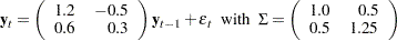The following statements compute the roots of characteristic function, compute the five lags of cross-covariance matrices, generate 100 observations simulated data, and evaluate the log-likelihood function of the VAR(1) model:

proc iml;
/* Stationary VAR(1) model */
sig = {1.0  0.5, 0.5 1.25};
phi = {1.2 -0.5, 0.6 0.3};
call varmasim(yt,phi) sigma=sig n=100 seed=3243; 
call vtsroot(root,phi); 
print root;
call varmacov(crosscov,phi) sigma=sig lag=5; 
lag = {'0','','1','','2','','3','','4','','5',''}; 
print lag crosscov;
call varmalik(lnl,yt,phi) sigma=sig; 
print lnl;

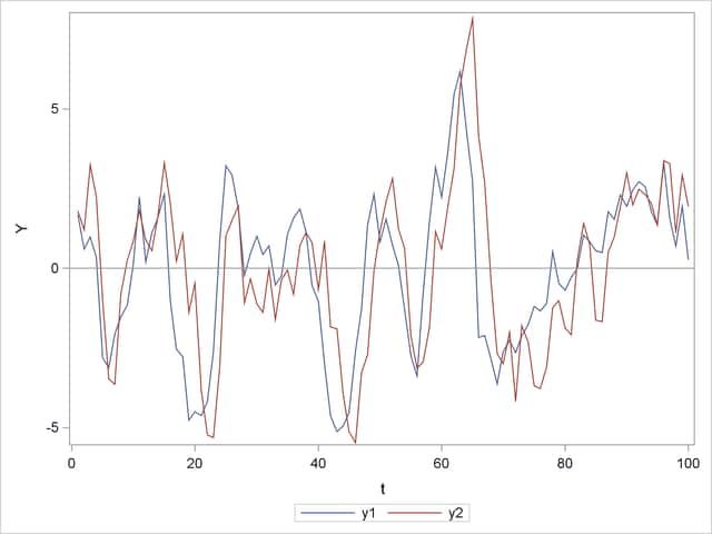
Output 13.4.3 Plot of Generated VAR(1) Process (VARMASIM)

The stationary VAR(1) processes show in Figure 13.4.3.

Output 13.4.4 Roots of VAR(1) Model (VTSROOT)

root
0.75	0.3122499	0.8124038	0.3945069	22.603583
0.75	-0.31225	0.8124038	-0.394507	-22.60358

In Figure 13.4.4, the first column is the real part ( $\text{[math]}$ ) of the root of the characteristic function and the second one is the imaginary part ( $\text{[math]}$ ). The third column is the modulus, the squared root of $\text{[math]}$ . The fourth column is $\text{[math]}$ and the last one is the degree. Since moduli are less than one from the third column, the series is obviously stationary.

Output 13.4.5 Cross-covariance Matrices of VAR(1) Model (VARMACOV)

lag	crosscov
0	5.3934173	3.8597124
	3.8597124	5.0342051
1	4.5422445	4.3939641
	2.1145523	3.826089
2	3.2537114	4.0435359
	0.6244183	2.4165581
3	1.8826857	3.1652876
	-0.458977	1.0996184
4	0.676579	2.0791977
	-1.100582	0.0544993
5	-0.227704	1.0297067
	-1.347948	-0.643999

In each matrix in Figure 13.4.5, the diagonal elements are corresponding to the autocovariance functions of each time series. The off-diagonal elements are corresponding to the cross-covariance functions of between two series.

Output 13.4.6 Log-Likelihood function of VAR(1) Model (VARMALIK)

lnl
-113.4708
2.5058678
224.43567

In Figure 13.4.6, the first row is the value of log-likelihood function; the second row is the sum of log determinant of the innovation variance; the last row is the weighted sum of squares of residuals.

Nonstationary VAR Process

Generate the process following the error correction model with a cointegrated rank of 1:

$\text{[math]}$

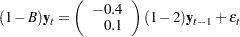with

$\text{[math]}$

The following statements compute the roots of characteristic function and generate simulated data.

proc iml;
/* Nonstationary  model */
sig = 100*i(2);
phi = {0.6 0.8, 0.1 0.8};
call varmasim(yt,phi) sigma=sig n=100 seed=1324; 
call vtsroot(root,phi); 
print root;

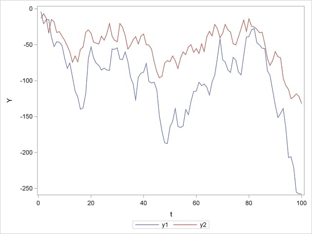
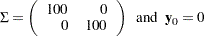
Output 13.4.7 Plot of Generated Nonstationary Vector Process (VARMASIM)

The nonstationary processes are shown in Figure 13.4.7 and have a comovement.

Output 13.4.8 Roots of Nonstationary VAR(1) Model (VTSROOT)

root
1	0	1	0	0
0.4	0	0.4	0	0

In Figure 13.4.8, the first column is the real part ( $\text{[math]}$ ) of the root of the characteristic function and the second one is the imaginary part ( $\text{[math]}$ ). The third column is the modulus, the squared root of $\text{[math]}$ . The fourth column is $\text{[math]}$ and the last one is the degree. Since the moduli are greater than equal to one from the third column, the series is obviously nonstationary.