Example 13.2 Kalman Filtering: Likelihood Function Evaluation
In the following example, the log-likelihood function of the SSM is computed by using prediction error decomposition. The annual real GNP series,  , can be decomposed as
where  is a trend component and
  is a white noise error with
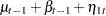
  . Refer to Nelson and Plosser (1982) for more details about these data. The trend component is assumed to be generated from the following stochastic equations:
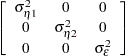
where  and
and  are independent white noise disturbances with
  and
and  .
.
It is straightforward to construct the SSM of the real GNP series.
where
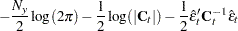
When the observation noise is normally distributed, the average log-likelihood function of the SSM is
where  is the mean square error matrix of the prediction error
  , such that
 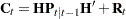 .
.
The LIK module computes the average log-likelihood function. First, the average log-likelihood function is computed by using the default initial values: Z0=0 and VZ0= I. The second call of module LIK produces the average log-likelihood function with the given initial conditions: Z0=0 and VZ0=
 I. You can notice a sizable difference between the uncertain initial condition (VZ0=I) and the almost deterministic initial condition (VZ0=I) in Output 13.2.1.
Finally, the first 15 observations of one-step predictions, filtered values, and real GNP series are produced under the moderate initial condition (VZ0= I). The data are the annual real GNP for the years 1909 to 1969. Here is the code:
 title 'Likelihood Evaluation of SSM';
 title2 'DATA: Annual Real GNP 1909-1969';
 data gnp;
    input y @@;
 datalines;
 116.8 120.1 123.2 130.2 131.4 125.6 124.5 134.3
 135.2 151.8 146.4 139.0 127.8 147.0 165.9 165.5
 179.4 190.0 189.8 190.9 203.6 183.5 169.3 144.2
 141.5 154.3 169.5 193.0 203.2 192.9 209.4 227.2
 263.7 297.8 337.1 361.3 355.2 312.6 309.9 323.7
 324.1 355.3 383.4 395.1 412.8 406.0 438.0 446.1
 452.5 447.3 475.9 487.7 497.2 529.8 551.0 581.1
 617.8 658.1 675.2 706.6 724.7
 ;
 run;
proc iml;
start lik(y,a,b,f,h,var,z0,vz0);
    nz = nrow(f);
    n = nrow(y);
    k = ncol(y);
    const = k*log(8*atan(1));
    if ( sum(z0 = .) | sum(vz0 = .) ) then
       call kalcvf(pred,vpred,filt,vfilt,y,0,a,f,b,h,var);
    else
       call kalcvf(pred,vpred,filt,vfilt,y,0,a,f,b,h,var,z0,vz0);
    et = y - pred*h`;
    sum1 = 0;
    sum2 = 0;
    do i = 1 to n;
       vpred_i = vpred[(i-1)*nz+1:i*nz,];
       et_i = et[i,];
       ft = h*vpred_i*h` + var[nz+1:nz+k,nz+1:nz+k];
       sum1 = sum1 + log(det(ft));
       sum2 = sum2 + et_i*inv(ft)*et_i`;
    end;
    return(-.5*const-.5*(sum1+sum2)/n);
finish;

use gnp;
read all var {y};
close gnp;

f = {1 1, 0 1};
h = {1 0};
a = j(nrow(f),1,0);
b = j(nrow(h),1,0);
var = diag(j(1,nrow(f)+ncol(y),1e-3));
/*-- initial values are computed --*/
z0 = j(1,nrow(f),.);
vz0 = j(nrow(f),nrow(f),.);
logl = lik(y,a,b,f,h,var,z0,vz0);
print 'No initial values are given', logl;
/*-- initial values are given --*/
z0 = j(1,nrow(f),0);
vz0 = 1e-3#i(nrow(f));
logl = lik(y,a,b,f,h,var,z0,vz0);
print 'Initial values are given', logl;
z0 = j(1,nrow(f),0);
vz0 = 10#i(nrow(f));
call kalcvf(pred0,vpred,filt0,vfilt,y,1,a,f,b,h,var,z0,vz0);

y0 = y;
free y;
y = j(16,1,0);
pred = j(16,2,0);
filt = j(16,2,0);
do i=1 to 16;
   y[i] = y0[i];
   pred[i,] = pred0[i,];
   filt[i,] = filt0[i,];
end;
print y pred filt;
quit;
Output 13.2.1
Average Log Likelihood of SSM
| No initial values are given |
Output 13.2.2 shows the observed data, the predicted state vectors, and the filtered state vectors for the first 16 observations.
Output 13.2.2
Filtering and One-Step Prediction
| 116.8 |
0 |
0 |
116.78832 |
0 |
| 120.1 |
116.78832 |
0 |
120.09967 |
3.3106857 |
| 123.2 |
123.41035 |
3.3106857 |
123.22338 |
3.1938303 |
| 130.2 |
126.41721 |
3.1938303 |
129.59203 |
4.8825531 |
| 131.4 |
134.47459 |
4.8825531 |
131.93806 |
3.5758561 |
| 125.6 |
135.51391 |
3.5758561 |
127.36247 |
-0.610017 |
| 124.5 |
126.75246 |
-0.610017 |
124.90123 |
-1.560708 |
| 134.3 |
123.34052 |
-1.560708 |
132.34754 |
3.0651076 |
| 135.2 |
135.41265 |
3.0651076 |
135.23788 |
2.9753526 |
| 151.8 |
138.21324 |
2.9753526 |
149.37947 |
8.7100967 |
| 146.4 |
158.08957 |
8.7100967 |
148.48254 |
3.7761324 |
| 139 |
152.25867 |
3.7761324 |
141.36208 |
-1.82012 |
| 127.8 |
139.54196 |
-1.82012 |
129.89187 |
-6.776195 |
| 147 |
123.11568 |
-6.776195 |
142.74492 |
3.3049584 |
| 165.9 |
146.04988 |
3.3049584 |
162.36363 |
11.683345 |
| 165.5 |
174.04698 |
11.683345 |
167.02267 |
8.075817 |