Call R Packages from PROC IML

You do not need to do anything special to call an R package. Provided that an R package is installed, you can call library(package) from inside a SUBMIT block to load the package. You can then call the functions in the package.

The example in this section calls an R package and imports the results into a SAS data set. This example is similar to the example in Creating Graphics in a SUBMIT Block, which calls the UNIVARIATE procedure to create a kernel density estimate. The program in this section consists of the following steps:

1. Define the data and transfer the data to R.

2. Call R functions to analyze the data.

3. Transfer the results of the analysis into SAS/IML vectors.

1. Define the data in the SAS/IML vector q and then transfer the data to R by using the ExportMatrixToR subroutine. In R, the data are stored in a vector named rq.

   proc iml;
   q = {3.7, 7.1, 2, 4.2, 5.3, 6.4, 8, 5.7, 3.1, 6.1, 4.4, 5.4, 9.5, 11.2};
   RVar = "rq";
   call ExportMatrixToR( q, RVar );
   

2. Load the KernSmooth package. Because the functions in the KernSmooth package do not handle missing values, the nonmissing values in q must be copied to a matrix p. (There are no missing values in this example.) The Sheather-Jones plug-in bandwidth is computed by calling the dpik function in the KernSmooth package. This bandwidth is used in the bkde function (in the same package) to compute a kernel density estimate.

   submit RVar / R;
      library(KernSmooth)
      idx <-which(!is.na(&RVar))        # must exclude missing values (NA)
      p <- &RVar[idx]                   #    from KernSmooth functions
      h = dpik(p)                       # Sheather-Jones plug-in bandwidth
      est <- bkde(p, bandwidth=h)       # est has 2 columns
   endsubmit;
   

3. Copy the results into a SAS data set or a SAS/IML matrix, and perform additional computations. For example, the following statements use the trapezoidal rule to numerically estimate the density that is contained in the tail of the density estimate of the data:

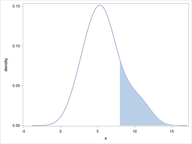
   call ImportMatrixFromR( m, "est" );
   /* estimate the density for q >= 8 */
   x = m[,1];                /* x values for density */  
   idx = loc( x>=8 );        /* find values x >= 8 */
   y = m[idx, 2];            /* extract corresponding density values */
   
   /* Use the trapezoidal rule to estimate the area under the density curve.
      The area of a trapezoid with base w and heights h1 and h2 is 
      w*(h1+h2)/2. */
   w = m[2,1] - m[1,1];      
   h1 = y[1:nrow(y)-1];      
   h2 = y[2:nrow(y)];
   Area = w * sum(h1+h2) / 2;
   print Area;
   

   The numerical estimate for the conditional density is shown in Figure 11.5. The estimate is shown graphically in Figure 11.6, where the conditional density corresponds to the shaded area in the figure. Figure 11.6 was created by using the SGPLOT procedure to display the density estimate computed by the R package.

   Figure 11.5 Computation That Combines SAS/IML and R Computations

   Area
   0.2118117

   
   

Figure 11.6 Estimated Density for