| Windows and Viewports |
A window defines a rectangular area in world coordinates. You define a window with a GWINDOW statement. You can define the window to be larger than, the same size as, or smaller than the actual range of data values, depending on whether you want to show all of the data or only part of the data.
A viewport defines in normalized coordinates a rectangular area on the display device where the image of the data appears. You define a viewport with the GPORT command. You can have your graph take up the entire display device or show it in only a portion, say the upper-right part.
Mapping Windows to Viewports
A window and a viewport are related by the linear transformation that maps the window onto the viewport. A line segment in the window is mapped to a line segment in the viewport such that the relative positions are preserved.
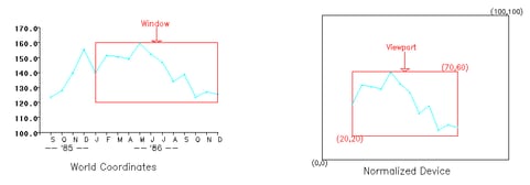
You do not have to display all of your data in a graph. In Figure 15.4, the graph on the left displays all of the ACME stock data, and the graph on the right displays only a part of the data. Suppose that you wanted to graph only the last 10 years of the stock data—say, from 1977 to 1986. You would want to define a window where the YEAR axis ranges from 77 to 86, while the PRICE axis could range from 120 to 160. Figure 15.4 shows stock prices in a window defined for data from 1977 to 1986 along the horizontal direction and from 120 to 160 along the vertical direction. The window is mapped to a viewport defined by the points (20,20) and (70,60). The appropriate GPORT and GWINDOW specifications are as follows:
   call gwindow({77 120, 86 160});
   call gport({20 20, 70 60});
The window, in effect, defines the portion of the graph that is to be displayed in world coordinates, and the viewport specifies the area on the device on which the image is to appear.
Understanding Windows
Because the default world coordinate system ranges from (0,0) to (100,100), you usually need to define a window in order to set the world coordinates that correspond to your data. A window specifies which part of the data in world coordinate space is to be shown. Sometimes you want all of the data shown; other times, you want to show only part of the data.
A window is defined by an array of four numbers, which define a rectangular area. You define this area by specifying the world coordinates of the lower-left and upper-right corners in the GWINDOW statement, which has the following general form:
- CALL GWINDOW (minimum-x minimum-y maximum-x maximum-y) ;
The argument can be either a matrix or a literal. The order of the elements is important. The array of coordinates can be a  ,
,  , or
, or  matrix. These coordinates can be specified as matrix literals or as the name of a numeric matrix that contains the coordinates. If you do not define a window, the default is to assume both
  and
and  range between 0 and 100.
In summary, a window
defines the portion of the graph that appears in the viewport
is a rectangular area
is defined by an array of four numbers
is defined in world coordinates
scales the data relative to world coordinates
In the previous example, the variable YEAR ranges from 1971 to 1986, while PRICE ranges from 123.625 to 159.50. Because the data do not fit nicely into the default, you want to define a window that reflects the ranges of the variables YEAR and PRICE. To draw the graph of these data to scale, you can let the YEAR axis range from 70 to 87 and the PRICE axis range from 100 to 200. Use the following statements to draw the graph, shown in Figure 15.5.
   call gstart;
   xbox={0 100 100 0};
   ybox={0 0 100 100};
   call gopen("stocks1");        /* begin new graph STOCKS1 */
   call gset("height", 2.0);
   year=do(71,86,1);                     /* initialize YEAR */
   price={123.75 128.00 139.75          /* initialize PRICE */
          155.50 139.750 151.500
          150.375 149.125 159.500
          152.375 147.000 134.125
          138.750 123.625 127.125
          125.50};
   call gwindow({70 100 87 200});                /* define window */
   call gpoint(year,price,"diamond","green"); /* graph the points */
   call gdraw(year,price,1,"green");            /* connect points */
   call gshow;                                  /* show the graph */
In the following example, you perform several steps that you did not do with the previous graph:
You associate the name STOCKS1 with this graphics segment in the GOPEN command.
You define a window that reflects the actual ranges of the data with a GWINDOW command.
You associate a plotting symbol, the diamond, and the color green with the GPOINT command.
You connect the points with line segments with the GDRAW command. The GDRAW command requests that the line segments be drawn in style 1 and be green.
Understanding Viewports
A viewport specifies a rectangular area on the display device where the graph appears. You define this area by specifying the normalized coordinates, the lower-left corner and the upper-right corner, in the GPORT statement, which has the following general form:
- CALL GPORT (minimum-x minimum-y maximum-x maximum-y) ;
The argument can be either a matrix or a literal. Note that both and must range between 0 and 100. As with the GWINDOW specification, you can give the coordinates either as a matrix literal enclosed in braces or as the name of a numeric matrix that contains the coordinates. The array can be a , , or matrix. If you do not define a viewport, the default is to span the entire display device.
In summary, a viewport
specifies where the image appears on the display
is a rectangular area
is specified by an array of four numbers
is defined in normalized coordinates
scales the data relative to the shape of the viewport
To display the stock price data in a smaller area on the display device, you must define a viewport. While you are at it, add some text to the graph. You can use the graph that you created and named STOCKS1 in this new graph. The following statements create the graph shown in Figure 15.6.
       /* module centers text strings */
   start gscenter(x,y,str);
      call gstrlen(len,str);               /* find string length */
      call gscript(x-len/2,y,str);                 /* print text */
   finish gscenter;

   call gopen("stocks2");                  /* open a new segment */
   call gset("font","swiss");              /* set character font */
   call gpoly(xbox,ybox);                  /* draw a border      */
   call gwindow({70 100,87 200});          /* define a window    */
   call gport({15 15,85 85});              /* define a viewport  */
   call ginclude("stocks1");          /* include segment STOCKS1 */
   call gxaxis({70 100},17,18, ,           /* draw x-axis        */
                ,"2.",1.5);
   call gyaxis({70 100},100,11, ,                 /* draw y-axis */
                ,"dollar5.",1.5);
   call gset("height",2.0);              /* set character height */
   call gtext(77,89,"Year");            /* print horizontal text */
   call gvtext(68,200,"Price");          /* print vertical text  */
   call gscenter(79,210,"ACME Stock Data");      /* print title  */
   call gshow;
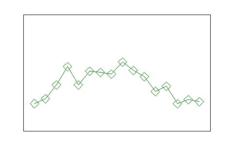
The following list describes the statements that generated this graph:
GOPEN begins a new graph and names it STOCKS2.
GPOLY draws a box around the display area.
GWINDOW defines the world coordinate space to be larger than the actual range of stock data values.
GPORT defines a viewport. It causes the graph to appear in the center of the display, with a border around it for text. The lower-left corner has coordinates (15,15) and the upper-right corner has coordinates (85,85).
GINCLUDE includes the graphics segment STOCKS1. This saves you from having to plot points you have already created.
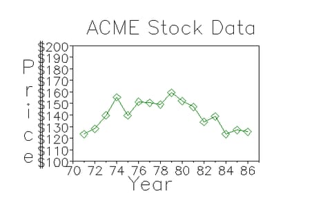
GXAXIS draws the
axis. It begins at the point (70,100) and is 17 units (years) long, divided with 18 tick marks. The axis tick marks are printed with the numeric 2.0 format, and they have a height of 1.5 units. GYAXIS draws the
axis. It also begins at (70,100) but is 100 units (dollars) long, divided with 11 tick marks. The axis tick marks are printed with the DOLLAR5.0 format and have a height of 1.5 units. GSET sets the text font to be Swiss and the height of the letters to be 2.0 units. The height of the characters has been increased because the viewport definition scales character sizes relative to the viewport.
GTEXT prints horizontal text. It prints the text string Year beginning at the world coordinate point (77,89).
GVTEXT prints vertical text. It prints the text string Price beginning at the world coordinate point (68,200).
GSCENTER runs the module to print centered text strings.
GSHOW displays the graph.
Changing Windows and Viewports
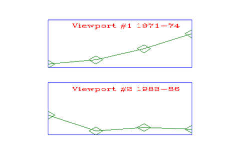
Windows and viewports can be changed for the graphics segment any time that the segment is active. Using the stock price example, you can first define a window for the data during the years 1971 to 1974 and map this to the viewport defined on the upper half of the normalized device; then you can redefine the window to enclose the data for 1983 to 1986 and map this to an area in the lower half of the normalized device. Notice how the shape of the viewport affects the shape of the curve. Changing the viewport can affect the height of any printed characters as well. In this case, you can modify the HEIGHT parameter.
The following statements generate the graph in Figure 15.7:
        /* figure 12.7  */
   reset clip;                          /* clip outside viewport */
   call gopen;                             /* open a new segment */
   call gset("color","blue");
   call gset("height",2.0);
   call gwindow({71 120,74 175});             /* define a window */
   call gport({20 55,80 90});               /* define a viewport */
   call gpoly({71 74 74 71},{120 120 170 170}); /* draw a border */
   call gscript(71.5,162,"Viewport #1 1971-74",,   /* print text */
                  ,3.0,"complex","red");
   call gpoint(year,price,"diamond","green");     /* draw points */
   call gdraw(year,price,1,"green");           /* connect points */
   call gblkvpd;
   call gwindow({83 120,86 170});           /* define new window */
   call gport({20 10,80 45});             /* define new viewport */
   call gpoly({83 86 86 83},{120 120 170 170});   /* draw border */
   call gpoint(year,price,"diamond","green");     /* draw points */
   call gdraw(year,price,1,"green");           /* connect points */
   call gscript(83.5,162,"Viewport #2 1983-86",,   /* print text */
                  ,3.0,"complex","red");
   call gshow;
The RESET CLIP command is necessary because you are graphing only a part of the data in the window. You want to clip the data that falls outside of the window. See the section Clipping Your Graphs for more about clipping. In this graph, you
open a new segment (GOPEN)
define the first window for the first four years’ data (GWINDOW)
define a viewport in the upper part of the display device (GPORT)
draw a box around the viewport (GPOLY)
add text (GSCRIPT)
graph the points and connect them (GPOINT and GDRAW)
define the second window for the last four years (GWINDOW)
define a viewport in the lower part of the display device (GPORT)
draw a box around the viewport (GPOLY)
graph the points and connect them (GPOINT and GDRAW)
add text (GSCRIPT)
display the graph (GSHOW)
Stacking Viewports
Viewports can be stacked; that is, a viewport can be defined relative to another viewport so that you have a viewport within a viewport.
A window or a viewport is changed globally through the IML graphics commands: the GWINDOW command for windows, and the GPORT, GPORTSTK, and GPORTPOP commands for viewports. When a window or viewport is defined, it persists across IML graphics commands until another window- or viewport-altering command is encountered. Stacking helps you define a viewport without losing the effect of a previously defined viewport. When a stacked viewport is popped, you are placed into the environment of the previous viewport.
Windows and viewports are associated with a particular segment; thus, they automatically become undefined when the segment is closed. A segment is closed whenever IML encounters a GCLOSE command or a GOPEN command. A window or a viewport can also be changed for a single graphics command. Either one can be passed as an argument to a graphics primitive, in which case any graphics output associated with the call is defined in the specified window or viewport. When a viewport is passed as an argument, it is stacked, or defined relative to the current viewport, and popped when the graphics command is complete.
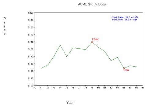
For example, suppose you want to create a legend that shows the low and peak points of the data for the ACME stock graph. Use the following statements to create a graphics segment showing this information:
   call gopen("legend");
   call gset('height',5);   /* enlarged to accommodate viewport later */
   call gset('font','swiss');
   call gscript(5,75,"Stock Peak:  159.5 in 1979");
   call gscript(5,65,"Stock Low:   123.6 in 1984");
   call gclose;
Use the following statements to create a segment that highlights and labels the low and peak points of the data:
     /* Highlight and label the low and peak points of the stock */
   call gopen("labels");
   call gwindow({70 100 87 200}); /* define window */
   call gpoint(84,123.625,"circle","red",4) ;
   call gtext(84,120,"LOW","red");
   call gpoint(79,159.5,"circle","red",4);
   call gtext(79,162,"PEAK","red");
   call gclose;
Next, open a new graphics segment and include the STOCK1 segment created earlier in the chapter, placing the segment in the viewport {10 10 90 90}. Here is the code:
   call gopen;
   call gportstk ({10 10 90 90}); /* viewport for the plot itself */
   call ginclude('stocks2');
To place the legend in the upper-right corner of this viewport, use the GPORTSTK command instead of the GPORT command to define the legend’s viewport relative to the one used for the plot of the stock data, as follows:
   call gportstk ({70 70 100 100});   /* viewport for the legend */
   call ginclude("legend");
Now pop the legend’s viewport to get back to the viewport of the plot itself and include the segment that labels and highlights the low and peak stock points. Here is the code:
   call gportpop;   /* viewport for the legend */
   call ginclude ("labels");
Finally, display the graph, as follows:
call gshow;