| Nonlinear Optimization Examples |
Example 14.6 Survival Curve for Interval Censored Data
In some studies, subjects are assessed only periodically for outcomes or responses of interest. In such situations, the occurrence times of these events are not observed directly; instead they are known to have occurred within some time interval. The times of occurrence of these events are said to be interval censored. A first step in the analysis of these interval censored data is the estimation of the distribution of the event occurrence times.
In a study with  subjects, denote the raw interval censored observations by
  . For the
  th subject, the event occurrence time
  lies in
  , where
  is the last assessment time at which there was no evidence of the event, and
  is the earliest time when a positive assessment was noted (if it was observed at all). If the event does not occur before the end of the study, is given a value larger than any assessment time recorded in the data.
A set of nonoverlapping time intervals  , is generated over which the survival curve
  is estimated. Refer to Peto (1973) and Turnbull (1976) for details. Assuming the independence of and , and also independence across subjects, the likelihood of the data
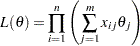
  can be constructed in terms of the pseudo-parameters
  . The conditional likelihood of
  is
is
 |
where  is 1 or 0 according to whether
  is a subset of . The maximum likelihood estimates,
  , yield an estimator
  of the survival function
  , which is given by
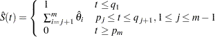 |
remains undefined in the intervals  where the function can decrease in an arbitrary way. The asymptotic covariance matrix of
  is obtained by inverting the estimated matrix of second partial derivatives of the negative log likelihood (Peto; 1973), (Turnbull; 1976). You can then compute the standard errors of the survival function estimators by the delta method and approximate the confidence intervals for survival function by using normal distribution theory.
The following code estimates the survival curve for interval censored data. As an illustration, consider an experiment to study the onset of a special kind of palpable tumor in mice. Forty mice exposed to a carcinogen were palpated for the tumor every two weeks. The times to the onset of the tumor are interval censored data. These data are contained in the data set CARCIN. The variable L represents the last time the tumor was not yet detected, and the variable R represents the first time the tumor was palpated. Three mice died tumor free, and one mouse was tumor free by the end of the 48-week experiment. The times to tumor for these four mice were considered right censored, and they were given an R value of 50 weeks.
data carcin;
   input id l r @@;
   datalines;
   1  20  22    11  30  32     21  22  24    31  34  36
   2  22  24    12  32  34     22  22  24    32  34  36
   3  26  28    13  32  34     23  28  30    33  36  38
   4  26  28    14  32  34     24  28  30    34  38  40
   5  26  28    15  34  36     25  32  34    35  38  40
   6  26  28    16  36  38     26  32  34    36  42  44
   7  28  30    17  42  44     27  32  34    37  42  44
   8  28  30    18  30  50     28  32  34    38  46  48
   9  30  32    19  34  50     29  32  34    39  28  50
  10  30  32    20  20  22     30  32  34    40  48  50
   ;

proc iml;
   use carcin;
   read all var{l r};
   nobs= nrow(l);
  /*********************************************************
      construct the nonoverlapping intervals (Q,P) and
      determine the number of pseudo-parameters (NPARM)
   *********************************************************/
   pp= unique(r); npp= ncol(pp);
   qq= unique(l); nqq= ncol(qq);
   q= j(1,npp, .);
   do;
      do i= 1 to npp;
         do j= 1 to nqq;
            if ( qq[j] < pp[i] ) then q[i]= qq[j];
         end;
         if q[i] = qq[nqq] then goto lab1;
      end;
   lab1:
   end;

   if i > npp then nq= npp;
   else            nq= i;
   q= unique(q[1:nq]);
   nparm= ncol(q);
   p= j(1,nparm, .);
   do i= 1 to nparm;
      do j= npp to 1 by -1;
         if ( pp[j] > q[i] ) then p[i]= pp[j];
      end;
   end;

  /********************************************************
      generate the X-matrix for the likelihood
   ********************************************************/
   _x= j(nobs, nparm, 0);
   do j= 1 to nparm;
      _x[,j]= choose(l <= q[j]  & p[j] <= r, 1, 0);
   end;

  /********************************************************
     log-likelihood function (LL)
   ********************************************************/
   start LL(theta) global(_x,nparm);
      xlt= log(_x * theta`);
      f= xlt[+];
      return(f);
   finish LL;

  /********************************************************
     gradient vector (GRAD)
   *******************************************************/
   start GRAD(theta) global(_x,nparm);
      g= j(1,nparm,0);
      tmp= _x # (1 /  (_x * theta`) );
      g= tmp[+,];
      return(g);
   finish GRAD;

  /*************************************************************
     estimate the pseudo-parameters using quasi-newton technique
   *************************************************************/
   /* options */
   optn= {1 2};

   /* constraints */
   con= j(3, nparm + 2, .);
   con[1, 1:nparm]= 1.e-6;
   con[2:3, 1:nparm]= 1;
   con[3,nparm + 1]=0;
   con[3,nparm + 2]=1;

   /* initial estimates */
   x0= j(1, nparm, 1/nparm);

   /* call the optimization routine */
   call nlpqn(rc,rx,"LL",x0,optn,con,,,,"GRAD");

  /*************************************************************
    survival function estimate (SDF)
   ************************************************************/
   tmp1= cusum(rx[nparm:1]);
   sdf= tmp1[nparm-1:1];

  /*************************************************************
    covariance matrix of the first nparm-1 pseudo-parameters (SIGMA2)
   *************************************************************/
   mm= nparm - 1;
   _x= _x - _x[,nparm] * (j(1, mm, 1) || {0});
   h= j(mm, mm, 0);
   ixtheta= 1 / (_x * ((rx[,1:mm]) || {1})`);
   if _zfreq then
      do i= 1 to nobs;
         rowtmp= ixtheta[i] # _x[i,1:mm];
         h= h + (_freq[i] # (rowtmp` * rowtmp));
      end;
   else do i= 1 to nobs;
      rowtmp= ixtheta[i] # _x[i,1:mm];
      h= h + (rowtmp` * rowtmp);
   end;
   sigma2= inv(h);

  /*************************************************************
    standard errors of the estimated survival curve (SIGMA3)
   *************************************************************/
   sigma3= j(mm, 1, 0);
   tmp1= sigma3;
   do i= 1 to mm;
      tmp1[i]= 1;
      sigma3[i]= sqrt(tmp1` * sigma2 * tmp1);
   end;

  /*************************************************************
    95% confidence limits for the survival curve (LCL,UCL)
   *************************************************************/
  /* confidence limits */
   tmp1= probit(.975);
   *print tmp1;
   tmp1= tmp1 * sigma3;
   lcl= choose(sdf > tmp1, sdf - tmp1, 0);
   ucl= sdf + tmp1;
   ucl= choose( ucl > 1., 1., ucl);

  /*************************************************************
    print estimates of pseudo-parameters
   *************************************************************/
   reset center noname;
   q= q`;
   p= p`;
   theta= rx`;
   print ,"Parameter Estimates", ,q[colname={q}] p[colname={p}]
         theta[colname={theta} format=12.7],;

  /*************************************************************
    print survival curve estimates and confidence limits
   *************************************************************/
   left= {0} // p;
   right= q // p[nparm];
   sdf= {1} // sdf // {0};
   lcl= {.} // lcl //{.};
   ucl= {.} // ucl //{.};
   print , "Survival Curve Estimates and 95% Confidence Intervals", ,
         left[colname={left}] right[colname={right}]
         sdf[colname={estimate} format=12.4]
         lcl[colname={lower} format=12.4]
         ucl[colname={upper} format=12.4];
The iteration history produced by the NLPQN subroutine is shown in Output 14.6.1.
| Optimization Start | |||
|---|---|---|---|
| Active Constraints | 1 | Objective Function | -93.3278404 |
| Max Abs Gradient Element | 65.361558529 | ||
| Iteration | Restarts | Function Calls |
Active Constraints |
Objective Function |
Objective Function Change |
Max Abs Gradient Element |
Step Size |
Slope of Search Direction |
||
|---|---|---|---|---|---|---|---|---|---|---|
| 1 | 0 | 3 | 1 | -88.51201 | 4.8158 | 16.6594 | 0.0256 | -305.2 | ||
| 2 | 0 | 4 | 1 | -87.42665 | 1.0854 | 10.8769 | 1.000 | -2.157 | ||
| 3 | 0 | 5 | 1 | -87.27408 | 0.1526 | 5.4965 | 1.000 | -0.366 | ||
| 4 | 0 | 7 | 1 | -87.17314 | 0.1009 | 2.2856 | 2.000 | -0.113 | ||
| 5 | 0 | 8 | 1 | -87.16611 | 0.00703 | 0.3444 | 1.000 | -0.0149 | ||
| 6 | 0 | 10 | 1 | -87.16582 | 0.000287 | 0.0522 | 1.001 | -0.0006 | ||
| 7 | 0 | 12 | 1 | -87.16581 | 9.128E-6 | 0.00691 | 1.133 | -161E-7 | ||
| 8 | 0 | 14 | 1 | -87.16581 | 1.712E-7 | 0.00101 | 1.128 | -303E-9 |
The estimates of the pseudo-parameter for the nonoverlapping intervals are shown in Output 14.6.2.
The survival curve estimates and confidence intervals are displayed in Output 14.6.3.
| LEFT | RIGHT | ESTIMATE | LOWER | UPPER |
|---|---|---|---|---|
| 0 | 20 | 1.0000 | . | . |
| 22 | 22 | 0.9500 | 0.8825 | 1.0000 |
| 24 | 26 | 0.8750 | 0.7725 | 0.9775 |
| 28 | 28 | 0.7750 | 0.6456 | 0.9044 |
| 30 | 30 | 0.6717 | 0.5252 | 0.8182 |
| 32 | 32 | 0.5911 | 0.4363 | 0.7458 |
| 34 | 34 | 0.3493 | 0.1973 | 0.5013 |
| 36 | 36 | 0.2619 | 0.1194 | 0.4045 |
| 38 | 38 | 0.2037 | 0.0720 | 0.3355 |
| 40 | 42 | 0.1455 | 0.0293 | 0.2617 |
| 44 | 46 | 0.0582 | 0.0000 | 0.1361 |
| 48 | 48 | 0.0291 | 0.0000 | 0.0852 |
| 50 | 50 | 0.0000 | . | . |
In this program, the quasi-Newton technique is used to maximize the likelihood function. You can replace the quasi-Newton routine by other optimization routines, such as the NLPNRR subroutine, which performs Newton-Raphson ridge optimization, or the NLPCG subroutine, which performs conjugate gradient optimization. Depending on the number of parameters and the number of observations, these optimization routines do not perform equally well. For survival curve estimation, the quasi-Newton technique seems to work fairly well since the number of parameters to be estimated is usually not too large.
Copyright © SAS Institute, Inc. All Rights Reserved.