| Language Reference |
| ORPOL Function |
The ORPOL function generates orthogonal polynomials on a discrete set of points.
The arguments to the ORPOL function are as follows:
- x
is an
 vector of values on which the polynomials are to be defined.
 - maxdegree
specifies the maximum degree polynomial to be computed. If maxdegree is omitted, the default value is
 . If weights is specified, maxdegree must also be specified.
 - weights
specifies an
vector of nonnegative weights associated with the points in x. If you specify weights, you must also specify maxdegree. If maxdegree is not specified or is specified incorrectly, the default weights (all weights are 1) are used.
The ORPOL matrix function generates orthogonal polynomials evaluated at the  points contained in x by using the algorithm of Emerson (1968). The result is a column-orthonormal matrix
  with rows and maxdegree
 columns such that
 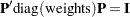 . The result of evaluating the polynomial of degree
  at the
  th element of x is stored in
  .
.
The maximum number of nonzero orthogonal polynomials ( ) that can be computed from the vector and the weights is the number of distinct values in the vector, ignoring any value associated with a zero weight.
The polynomial of maximum degree has degree of  . If the value of maxdegree exceeds , then columns
  ,
,  ,..., maxdegree of the result are set to 0. In this case,
 |
The following statement results in a matrix with three orthogonal columns:
  x = T(1:5);
  P = orpol(x,2);

                               P

                  0.4472136 -0.632456 0.5345225
                  0.4472136 -0.316228 -0.267261
                  0.4472136         0 -0.534522
                  0.4472136 0.3162278 -0.267261
                  0.4472136 0.6324555 0.5345225
The first column is a polynomial of degree 0 (a constant polynomial) evaluated at each point of  . The second column is a polynomial of degree 1 evaluated at each point of . The third column is a polynomial of degree 2 evaluated at each point of .
Normalization of the Polynomials
The columns of are orthonormal with respect to the inner product
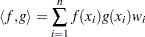 |
as shown by the following statements:
   start InnerProduct(f,g,w);
      h = f#g#w;
      return (h[+]);
   finish;

   /* Verify orthonormal */
   reset fuzz;         /* print tiny numbers as zero */
   w = j(ncol(x),1,1); /* default weight is all ones */
   do i = 1 to 3;
      do j = 1 to i;
         InnerProd = InnerProduct(P[,i], P[,j], w );
         print i j InnerProd;
      end;
   end;
Some reference books on orthogonal polynomials do not normalize the columns of the matrix that represents the orthogonal polynomials. For example, a textbook might give the following as a fourth-degree polynomial evaluated on evenly spaced data:
   textbookPoly = { 1 -2  2 -1  1,
                    1 -1 -1  2 -4,
                    1  0 -2  0  6,
                    1  1 -1 -2 -4,
                    1  2  2  1  1 };
To compare this representation to the normalized representation that ORPOL produces, use the following program:
   /* Normalize the columns of textbook representation */
   normalPoly = textbookPoly;
   do i = 1 to ncol( normalPoly );
      v = normalPoly[,i];
      norm = sqrt(v[##]);
      normalPoly[,i] = v / norm;
   end;

   /* Compare the normalized matrix with ORPOL */
   x = T(1:5); /* Any evenly spaced data gives the same answer */
   imlPoly = orpol( x, 4 );

   diff = imlPoly - normalPoly;
   maxDiff = abs(diff)[<>];
   reset fuzz; /* print tiny numbers as zero */
   print maxDiff;

            MAXDIFF

               0
Polynomial Regression
A typical use for orthogonal polynomials is to fit a polynomial to a set of data. Given a set of points  ,
,  , the classical theory of orthogonal polynomials says that the best approximating polynomial of degree
  is given by
 |
where  and where
  is the th column of the matrix returned by ORPOL. But the matrix is orthonormal with respect to the inner product, so
  for all . Thus you can easily compute a regression onto the span of polynomials.
In the following program, the weight vector is used to overweight or underweight particular data points. The researcher has reasons to doubt the accuracy of the first measurement. The last data point is also underweighted because it is a leverage point and is believed to be an outlier. The second data point was measured twice and is overweighted. (Rerunning the program with a weight vector of all ones, and examining the new values of the fit variable is a good way to understand the effect of the weight vector.)
   x = {0.1, 2,   3,  5,    8,   10, 20};
   y = {0.5, 1, 0.1, -1, -0.5, -0.8, 0.1};

   /* The second measurement was taken twice.
      The first and last data points are underweighted
      because of uncertainty in the measurements.  */
   w = {0.5, 2,   1,  1,    1,    1, 0.2};
   maxDegree = 4;
   P = orpol(x,maxDegree,w);

   /* The best fit by a polynomial of degree k is
      Sum c_i P_i  where c_i = <f,P_i> */
   c = j(1,maxDegree+1);
   do i = 1 to maxDegree+1;
      c[i] = InnerProduct(y,P[,i],w);
   end;

   FitResults = j(maxDegree+1,2);
   do k = 1 to maxDegree+1;
      fit = P[,1:k] * c[1:k];
      resid = y - fit;
      FitResults[k,1] = k-1;       /* degree of polynomial */
      FitResults[k,2] = resid[##]; /* sum of square errors */
   end;
   print FitResults[colname={"Degree" "SSE"}];
The results of this program are as follows:
     FITRESULTS
   Degree       SSE

        0 3.1733014
        1 4.6716722
        2 1.3345326
        3 1.3758639
        4 0.8644558
Testing Linear Hypotheses
ORPOL can also be used to test linear hypotheses. Suppose you have an experimental design with  factor levels. (The factor levels can be equally or unequally spaced.) At the th level, you record
  observation,
  . If
. If  , then the design is said to be balanced, otherwise it is unbalanced. You want to fit a polynomial model to the data and then ask how much variation in the data is explained by the linear component, how much variation is explained by the quadratic component after the linear component is taken into account, and so on for the cubic, quartic, and higher-level components.
To be completely concrete, suppose you have four factor levels (1, 4, 6, and 10) and that you record seven measurements at first level, two measurements at the second level, three measurements at the third level, and four measurements at the fourth level. This is an example of an unbalanced and unequally spaced factor-level design. The following program uses orthogonal polynomials to compute the Type I sum of squares for the linear hypothesis. (The program works equally well for balanced designs and for equally spaced factor levels.)
The program calls ORPOL to generate the orthogonal polynomial matrix , and uses it to form the Type I hypothesis matrix  . The program then uses the DESIGN function to generate
  , the design matrix associated with the experiment. The program then computes
  , the estimated parameters of the linear model.
Since was expressed in terms of the orthogonal polynomial matrix , the computations involved in forming the Type I sum of squares are considerably simplified.
/* unequally spaced and unbalanced factor levels */
levels = {
1,1,1,1,1,1,1,
4,4,
6,6,6,
10,10,10,10};
/* data for y. Make sure the data are sorted
according to the factor levels */
y = {
2.804823, 0.920085, 1.396577, -0.083318,
3.238294, 0.375768, 1.513658, /* level 1 */
3.913391, 3.405821, /* level 4 */
6.031891, 5.262201, 5.749861, /* level 6 */
10.685005, 9.195842, 9.255719, 9.204497 /* level 10 */
};
a = {1,4,6,10}; /* spacing */
trials = {7,2,3,4}; /* sample sizes */
maxDegree = 3; /* model with Intercept,a,a##2,a##3 */
P = orpol(a,maxDegree,trials);
/* Test linear hypotheses:
How much variation is explained by the
i_th polynomial component after components
0..(i-1) have been taken into account? */
/* the columns of L are the coefficients of the
orthogonal polynomial contrasts */
L = diag(trials)*P;
/* form design matrix */
x = design(levels);
/* compute b, the estimated parameters of the
linear model. b is the mean of the y values
at each level.
b = ginv(x'*x) * x` * y
but since x is the output from DESIGN, then
x`*x = diag(trials) and so
ginv(x`*x) = diag(1/trials) */
b = diag(1/trials)*x`*y;
/* (L`*b)[i] is the best linear unbiased estimated
(BLUE) of the corresponding orthogonal polynomial
contrast */
blue = L`*b;
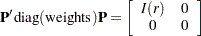
/* the variance of (L`*b) is
var(L`*b) = L`*ginv(x`*x)*L
=[P`*diag(trials)]*diag(1/trials)*[diag(trials)*P]
= P`*diag(trials)*P
= Identity (by definition of P)
so therefore the standardized square of
(L`*b) is computed as
SS1[i] = (blue[i]*blue[i])/var(L`*b)[i,i])
= (blue[i])##2 */
SS1 = blue # blue;
rowNames = {"Intercept" "Linear" "Quadratic" "Cubic"};
print SS1[rowname=rowNames format=11.7 label="Type I SS"];
The resulting output is as follows:
         Type I SS

   Intercept 331.8783538
   Linear    173.4756050
   Quadratic   0.4612604
   Cubic       0.0752106
This indicates that most of the variation in the data can be explained by a first-degree polynomial.
Generating Families of Orthogonal Polynomials
There are classical families of orthogonal polynomials (for example, Legendre, Laguerre, Hermite, and Chebyshev) that arise in the study of differential equations and mathematical physics. These "named" families are orthogonal on particular intervals  with respect to the inner product
 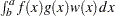 . The functions returned by ORPOL are different from these named families because ORPOL uses a different inner product. There are no built-in functions that can automatically generate these families; however, you can write a program to generate them.
Each named polynomial family  ,
,  satisfies a three-term recurrence relation of the form
 |
where the constants  ,
,  , and
, and  are relatively simple functions of
  . To generate these "named" families, use the three-term recurrence relation for the family. The recurrence relations are found in references such as Abramowitz and Stegun (1972) or Thisted (1988).
For example, the so-called Legendre polynomials (represented  for the polynomial of degree ) are defined on
  with the weight function
  . They are standardized by requiring that
  for all . Thus
  . The linear polynomial
  is orthogonal to
  so that
 |
which implies  . The standardization
  implies that
  . The remaining Legendre polynomials can be computed by looking up the three-term recurrence relation:
  ,
,  , and
, and  . The following program computes Legendre polynomials evaluated at a set of points.
maxDegree = 6;

/* evaluate polynomials at these points */
x = T( do(-1,1,0.05) );

/* define the standard Legendre Polynomials
   Using the 3-term recurrence with
   A[j]=0, B[j]=(2j-1)/j, and C[j]=(j-1)/j
   and the standardization P_j(1)=1
   which implies P_0(x)=1, P_1(x)=x. */
legendre = j(nrow(x), maxDegree+1);
legendre[,1] = 1; /* P_0 */
legendre[,2] = x; /* P_1 */

do j = 2 to maxDegree;
   legendre[,j+1] = (2*j-1)/j # x # legendre[,j] -
                      (j-1)/j # legendre[,j-1];
end;
Copyright © SAS Institute, Inc. All Rights Reserved.