| Wavelet Analysis |
Some Brief Mathematical Preliminaries
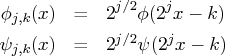
The discrete wavelet transform decomposes a function as a sum of basis
functions called wavelets. These basis functions have
the property that they can be obtained by dilating and translating
two basic types of wavelets known as the scaling function, or
father wavelet ![]() , and
the mother wavelet
, and
the mother wavelet ![]() . These translations and dilations are defined
as follows:
. These translations and dilations are defined
as follows:
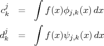
Conversely, if you know the detail and scaling coefficients at level
![]() , then you can obtain the scaling coefficients at level
, then you can obtain the scaling coefficients at level ![]() by using
the relationship
by using
the relationship
Suppose that you have data values
at ![]() equally spaced points
equally spaced points ![]() . It turns out that
the values
. It turns out that
the values ![]() are good approximations of the
scaling coefficients
are good approximations of the
scaling coefficients ![]() . Then, by using
the recurrence formula, you can find
. Then, by using
the recurrence formula, you can find ![]() and
and ![]() ,
,
![]() . The discrete wavelet transform of the
. The discrete wavelet transform of the ![]() at
level
at
level ![]() consists of the
consists of the ![]() scaling and
scaling and ![]() detail coefficients
at level
detail coefficients
at level ![]() . A technical point that arises is that
in applying the recurrence relationships to finite data, a few
values of the
. A technical point that arises is that
in applying the recurrence relationships to finite data, a few
values of the ![]() for
for ![]() or
or ![]() might be needed. One way to cope with this
difficulty is to extend the sequence
might be needed. One way to cope with this
difficulty is to extend the sequence ![]() to the left and right
by using some specified boundary treatment.
to the left and right
by using some specified boundary treatment.
Continuing by replacing the scaling coefficients at any
level ![]() by the scaling and detail coefficients at level
by the scaling and detail coefficients at level ![]() yields
a sequence of
yields
a sequence of ![]() coefficients
coefficients
This sequence is the finite discrete wavelet transform of the input
data ![]() . At any level
. At any level ![]() the finite dimensional approximation
of the function
the finite dimensional approximation
of the function ![]() is
is
Copyright © 2009 by SAS Institute Inc., Cary, NC, USA. All rights reserved.