Time Series Analysis and Examples

Getting Started

Consider a time series of length 100 from the ARMA(2,1) model

where the error series follows a normal with mean 10 and standard deviation 2.

The following statements generate the ARMA(2,1) model, compute 10 lags of its autocovariance functions, and calculate its log-likelihood function and residuals:

  
    proc iml; 
       /* ARMA(2,1) model */ 
       phi = {1 -0.5 0.04}; 
       theta = {1 0.25}; 
       mu = 10; 
       sigma = 2; 
       nobs = 100; 
       seed = 3456; 
       lag = 10; 
       yt = armasim(phi, theta, mu, sigma, nobs, seed); 
       print yt; 
       call armacov(autocov, cross, convol, phi, theta, lag); 
       autocov = autocov`; 
       cross = cross`; 
       convol = convol`; 
       lag = (0:lag-1)`; 
       print autocov cross convol; 
       call armalik(lnl, resid, std, yt, phi, theta); 
       print lnl resid std;
 

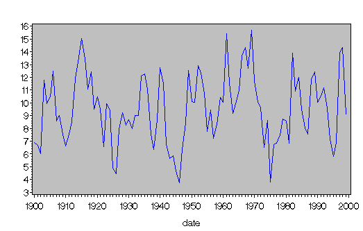
Figure 10.1: Plot of Generated ARMA(2,1) Process (ARMASIM)

The ARMASIM function generates the data shown in Figure 10.1.

LAG AUTOCOV CROSS CONVOL 0 1.6972803 1.1875 1.0625 1 1.0563848 0.25 0.25 2 0.4603012     3 0.1878952     4 0.0755356     5 0.030252     6 0.0121046     7 0.0048422     8 0.0019369     9 0.0007748

Figure 10.2: Autocovariance functions of ARMA(2,1) Model (ARMACOV)

In Figure 10.2, the ARMACOV subroutine prints the autocovariance functions of the ARMA(2,1) model and the covariance functions of the moving-average term with lagged values of the process and the autocovariance functions of the moving-average term.

LNL RESID STD -154.9148 5.2779797 1.3027971 22.034073 2.3491607 1.0197 0.5705918 2.3893996 1.0011951   8.4086892 1.0000746   2.200401 1.0000047   5.4127254 1.0000003   6.2756004 1   1.1944693 1   4.9425372 1   . .   . .

Figure 10.3: Log-Likelihood Function of ARMA(2,1) Model (ARMALIK)

The first column in Figure 10.3 shows the log-likelihood function, the estimate of the innovation variance, and the log of the determinant of the variance matrix. The next two columns are part of the results in the standardized residuals and the scale factors used to standardize the residuals.