Time Series Analysis and Examples

Nonstationary VAR Process

Generate the process following the error correction model with a cointegrated rank of 1:

with

The following statements compute the roots of characteristic function and generate simulated data.

  
    proc iml; 
       /* Nonstationary  model */ 
       sig = 100*i(2); 
       phi = {0.6 0.8, 0.1 0.8}; 
       call varmasim(yt,phi) sigma = sig n = 100 seed=1324; 
       call vtsroot(root,phi); print root; 
       print yt;
 

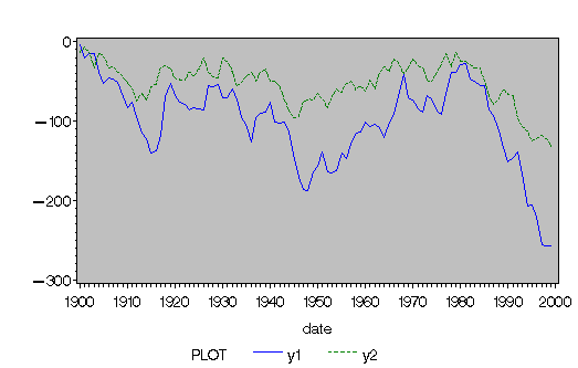
Figure 10.32: Plot of Generated Nonstationary Vector Process (VARMASIM)

The nonstationary processes are shown in Figure 10.32 and have a comovement.

ROOT 1 0 1 0 0 0.4 0 0.4 0 0

Figure 10.33: Roots of Nonstationary VAR(1) Model (VTSROOT)

In Figure 10.33, the first column is the real part () of the root of the characteristic function and the second one is the imaginary part (). The third column is the modulus, the squared root of . The fourth column is and the last one is the degree. Since the moduli are greater than equal to one from the third column, the series is obviously nonstationary.