Time Series Analysis and Examples: Example 10.2: Kalman Filtering: Likelihood Function Evaluation

Time Series Analysis and Examples

Example 10.2: Kalman Filtering: Likelihood Function Evaluation

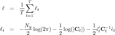
In the following example, the log-likelihood function of the SSM is computed by using prediction error decomposition. The annual real GNP series, , can be decomposed as

$y_t = \mu_t + \epsilon_t$

where $\mu_t$ is a trend component and $\epsilon_t$ is a white noise error with $\epsilon_t \sim (0, \sigma^2_\epsilon)$ . Refer to Nelson and Plosser (1982) for more details about these data. The trend component is assumed to be generated from the following stochastic equations:

$\mu_t & = & \mu_{t-1} + \beta_{t-1} + \eta_{1t} \ \beta_t & = & \beta_{t-1} + \eta_{2t}$

where $\eta_{1t}$ and $\eta_{2t}$ are independent white noise disturbances with $\eta_{1t} \sim (0, \sigma^2_{\eta_1})$ and $\eta_{2t} \sim (0, \sigma^2_{\eta_2})$ .

It is straightforward to construct the SSM of the real GNP series.

$y_t & = & {h}{z}_t + \epsilon_t \ {z}_t & = & {f}{z}_{t-1} + \eta_t$

where

${h}& = & (1, 0) \ {f}& = & [ 1 & 1 \ 0 & 1 ] \ {z}_t & = & (\mu_t, \beta... ...\eta 1} & 0 & 0 \ 0 & \sigma^2_{\eta 2} & 0 \ 0 & 0 & \sigma^2_\epsilon ]$

When the observation noise $\epsilon_t$ is normally distributed, the average log-likelihood function of the SSM is

$\ell & = & \frac{1}t \sum_{t=1}^t \ell_t \ \ell_t & = & -\frac{n_y}2\log(2\pi)... ...1}2\log(|{c}_t|) - \frac{1}2 \hat{\epsilon}^'_t {c}^{-1}_t \hat{\epsilon}_t$

where ${c}_t$ is the mean square error matrix of the prediction error $\hat{\epsilon}_t$ , such that ${c}_t = {h}{p}_{t| t-1} {h}^' + {{r}}_t$ .

The LIK module computes the average log-likelihood function. First, the average log-likelihood function is computed by using the default initial values: Z0=0 and VZ0=I. The second call of module LIK produces the average log-likelihood function with the given initial conditions: Z0=0 and VZ0= $10^{-3}$ I. You can notice a sizable difference between the uncertain initial condition (VZ0=I) and the almost deterministic initial condition (VZ0= $10^{-3}$ I) in Output 10.2.1.

Finally, the first 15 observations of one-step predictions, filtered values, and real GNP series are produced under the moderate initial condition (VZ0=10I). The data are the annual real GNP for the years 1909 to 1969. Here is the code:

  
    title 'Likelihood Evaluation of SSM'; 
    title2 'DATA: Annual Real GNP 1909-1969'; 
    data gnp; 
       input y @@; 
    datalines; 
       116.8 120.1 123.2 130.2 131.4 125.6 124.5 134.3 
       135.2 151.8 146.4 139.0 127.8 147.0 165.9 165.5 
       179.4 190.0 189.8 190.9 203.6 183.5 169.3 144.2 
       141.5 154.3 169.5 193.0 203.2 192.9 209.4 227.2 
       263.7 297.8 337.1 361.3 355.2 312.6 309.9 323.7 
       324.1 355.3 383.4 395.1 412.8 406.0 438.0 446.1 
       452.5 447.3 475.9 487.7 497.2 529.8 551.0 581.1 
       617.8 658.1 675.2 706.6 724.7 
       ; 
  
     proc iml; 
       start lik(y,a,b,f,h,var,z0,vz0); 
           nz = nrow(f); 
           n = nrow(y); 
           k = ncol(y); 
           const = k*log(8*atan(1)); 
           if ( sum(z0 = .) | sum(vz0 = .) ) then 
              call kalcvf(pred,vpred,filt,vfilt,y,0,a,f,b,h,var); 
           else 
              call kalcvf(pred,vpred,filt,vfilt,y,0,a,f,b,h,var,z0,vz0); 
           et = y - pred*h`; 
           sum1 = 0; 
           sum2 = 0; 
           do i = 1 to n; 
              vpred_i = vpred[(i-1)*nz+1:i*nz,]; 
              et_i = et[i,]; 
              ft = h*vpred_i*h` + var[nz+1:nz+k,nz+1:nz+k]; 
              sum1 = sum1 + log(det(ft)); 
              sum2 = sum2 + et_i*inv(ft)*et_i`; 
           end; 
           return(-.5*const-.5*(sum1+sum2)/n); 
       finish;

  
    start main; 
       use gnp; 
       read all var {y}; 
  
       f = {1 1, 0 1}; 
       h = {1 0}; 
       a = j(nrow(f),1,0); 
       b = j(nrow(h),1,0); 
       var = diag(j(1,nrow(f)+ncol(y),1e-3)); 
       /*-- initial values are computed --*/ 
       z0 = j(1,nrow(f),.); 
       vz0 = j(nrow(f),nrow(f),.); 
       logl = lik(y,a,b,f,h,var,z0,vz0); 
       print 'No initial values are given', logl; 
       /*-- initial values are given --*/ 
       z0 = j(1,nrow(f),0); 
       vz0 = 1e-3#i(nrow(f)); 
       logl = lik(y,a,b,f,h,var,z0,vz0); 
       print 'Initial values are given', logl; 
       z0 = j(1,nrow(f),0); 
       vz0 = 10#i(nrow(f)); 
       call kalcvf(pred,vpred,filt,vfilt,y,1,a,f,b,h,var,z0,vz0); 
       print y pred filt; 
    finish; 
    run;

Output 10.2.1: Average Log Likelihood of SSM

Likelihood Evaluation of SSM

DATA: Annual Real GNP 1909-1969

No initial values are given

LOGL
-26314.66

Initial values are given

LOGL
-91884.41

Output 10.2.2 shows the observed data, the predicted state vectors, and the filtered state vectors for the first 16 observations.

Output 10.2.2: Filtering and One-Step Prediction

Y	PRED		FILT
116.8	0	0	116.78832	0
120.1	116.78832	0	120.09967	3.3106857
123.2	123.41035	3.3106857	123.22338	3.1938303
130.2	126.41721	3.1938303	129.59203	4.8825531
131.4	134.47459	4.8825531	131.93806	3.5758561
125.6	135.51391	3.5758561	127.36247	-0.610017
124.5	126.75246	-0.610017	124.90123	-1.560708
134.3	123.34052	-1.560708	132.34754	3.0651076
135.2	135.41265	3.0651076	135.23788	2.9753526
151.8	138.21324	2.9753526	149.37947	8.7100967
146.4	158.08957	8.7100967	148.48254	3.7761324
139	152.25867	3.7761324	141.36208	-1.82012
127.8	139.54196	-1.82012	129.89187	-6.776195
147	123.11568	-6.776195	142.74492	3.3049584
165.9	146.04988	3.3049584	162.36363	11.683345
165.5	174.04698	11.683345	167.02267	8.075817

Top of Page