Time Series Analysis and Examples: Getting Started

Time Series Analysis and Examples

Getting Started

The measurement (or observation) equation can be written

${y}_t = {b}_t + {h}_t {z}_t + \epsilon_t$

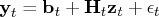
where ${b}_t$ is an

vector, ${h}_t$ is an

matrix, the sequence of observation noise $\epsilon_t$ is independent, ${z}_t$ is an

state vector, and ${y}_t$ is an

observed vector.

The transition (or state) equation is denoted as a first-order Markov process of the state vector.

${z}_{t+1} = {a}_t + {f}_t {z}_t + \eta_t$

where ${a}_t$ is an

vector, ${f}_t$ is an

transition matrix, and the sequence of transition noise $\eta_t$ is independent. This equation is often called a shifted transition equation because the state vector is shifted forward one time period. The transition equation can also be denoted by using an alternative specification

${z}_t = {a}_t + {f}_t {z}_{t-1} + \eta_t$

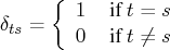
There is no real difference between the shifted transition equation and this alternative equation if the observation noise and transition equation noise are uncorrelated - that is, $e(\eta_t \epsilon^'_t) = 0$ . It is assumed that

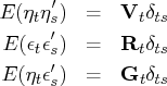
$e(\eta_t \eta^'_s) & = & {v}_t \delta_{ts} \ e(\epsilon_t \epsilon^'_s) & = & {{r}}_t \delta_{ts} \ e(\eta_t \epsilon^'_s) & = & {g}_t \delta_{ts} \$

where

$\delta_{ts} = \{ 1 & { if } t = s \ 0 & { if } t \neq s .$

De Jong (1991a) proposed a diffuse Kalman filter that can handle an arbitrarily large initial state covariance matrix. The diffuse initial state assumption is reasonable if you encounter the case of parameter uncertainty or SSM nonstationarity. The SSM of the diffuse Kalman filter is written

${y}_t & = & {x}_t \beta + {h}_t {z}_t + \epsilon_t \ {z}_{t+1} & = & {w}_t \bet... ...f}_t {z}_t + \eta_t \ {z}_0 & = & {a}+ {a}\delta \ \beta & = & {b}+ {b}\delta$

where $\delta$ is a random variable with a mean of $\mu$ and a variance of $\sigma^2\sigma$ . When $\sigma arrow \infty$ , the SSM is said to be diffuse.

The KALCVF call computes the one-step prediction ${z}_{t+1| t}$ and the filtered estimate ${z}_{t| t}$ , together with their covariance matrices ${p}_{t+1| t}$ and ${p}_{t| t}$ , using forward recursions. You can obtain the -step prediction ${z}_{t+k| t}$ and its covariance matrix ${p}_{t+k| t}$ with the KALCVF call. The KALCVS call uses backward recursions to compute the smoothed estimate ${z}_{t| t}$ and its covariance matrix ${p}_{t| t}$ when there are observations in the complete data.

The KALDFF call produces one-step prediction of the state and the unobserved random vector $\delta$ as well as their covariance matrices. The KALDFS call computes the smoothed estimate ${z}_{t| t}$ and its covariance matrix ${p}_{t| t}$ .

Top of Page