Sparse Matrix Algorithms

Example: Biconjugate Gradient Algorithm

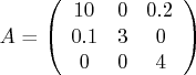
The biconjugate gradient algorithm is meant for general sparse linear systems. Matrix symmetry is no longer assumed, and a complete list of nonzero coefficients must be provided. Consider the following matrix:

with

The code for this example is as follows:

  
  
    /* biconjugate gradient algorithm */ 
  
    /*  value  row column */ 
    A = { 10    1     1, 
          3     2     2, 
          4     3     3, 
          0.1   2     1, 
          0.2   1     3 }; 
  
    /* vector of right-hand sides */ 
    b = {1, 1, 1}; 
  
    /* desired solution tolerance */ 
    tol = 1e-9; 
  
    /* maximum number of iterations */ 
    maxit = 10000; 
  
    /* allocate history/progress */ 
    hist = j(50, 1); 
  
    /* initial guess (optional) */ 
    start = {2, 3, 4}; 
  
    /* call biconjugate gradient subroutine */ 
    call itsolver ( 
       x, st, it,            /* output parameters */ 
       'bicg', a, b, 'milu', /* input parameters */ 
       tol,                  /* optional control parameters */ 
       maxit, 
       start, 
       hist); 
  
    /* Print results */ 
    print  x; 
    print st; 
    print it;
 

Here is the output:

  
                     X 
                     0.095 
                 0.3301667 
                      0.25 
  
                     ST 
                 1.993E-16 
  
                     IT 
                         3
 

It is important to observe the resultant tolerance in order to know how effective the solution is.