Nonlinear Optimization Examples: Kuhn-Tucker Conditions

Nonlinear Optimization Examples

Kuhn-Tucker Conditions

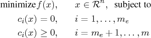
The nonlinear programming (NLP) problem with one objective function and constraint functions , which are continuously differentiable, is defined as follows:

${minimize} f(x), & & x \in {\cal r}^n, \; { subject to} \ c_i(x) = 0 , & & i = 1, ... ,m_e \ c_i(x) \ge 0 , & & i = m_e+1, ... ,m$

In the preceding notation,

is the dimension of the function

, and

is the number of equality constraints. The linear combination of objective and constraint functions

$l(x,\lambda) = f(x) - \sum_{i=1}^m \lambda_i c_i(x)$

is the Lagrange function, and the coefficients $\lambda_i$ are the Lagrange multipliers.

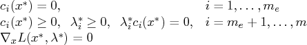
If the functions and are twice differentiable, the point is an isolated local minimizer of the NLP problem, if there exists a vector $\lambda^*=(\lambda_1^*, ... ,\lambda_m^*)$ that meets the following conditions:

Kuhn-Tucker conditions
$c_i(x^*) = 0 , & i = 1, ... ,m_e \ c_i(x^*) \ge 0 , \lambda_i^* \ge 0, \la... ..._i^* c_i(x^*) = 0 , & i = m_e+1, ... ,m \ \nabla_x l(x^*,\lambda^*) = 0$
second-order condition

Each nonzero vector $y \in {\cal r}^n$ with

$y^t \nabla_x c_i(x^*) = 0 i = 1, ... ,m_e ,\; { and } \forall i\in {m_e+1, ... ,m}; \lambda_i^* \gt 0$

satisfies

$y^t \nabla_x^2 l(x^*,\lambda^*) y \gt 0$

In practice, you cannot expect the constraint functions to vanish within machine precision, and determining the set of active constraints at the solution might not be simple.

Top of Page