Language Reference

FARMALIK Call

computes the log-likelihood function of an ARFIMA() model

CALL FARMALIK( lnl, series, d <, phi, theta, sigma, p, q, opt>);

The inputs to the FARMALIK subroutine are as follows:

series

specifies a time series (assuming mean zero).

d

specifies a fractional differencing order. This argument is required; the value of should be in the open interval excluding zero.

phi

specifies an -dimensional vector containing the autoregressive coefficients, where is the number of the elements in the subset of the AR order. The default is zero.

theta

specifies an -dimensional vector containing the moving-average coefficients, where is the number of the elements in the subset of the MA order. The default is zero.

sigma

specifies a variance of the innovation series. The default is one.

p

specifies the subset of the AR order. See the FARMACOV subroutine for additional details.

q

specifies the subset of the MA order. See the FARMACOV subroutine for additional details.

opt

specifies the method of computing the log-likelihood function.

opt=0

requests the conditional sum of squares function. This is the default.

opt=1

requests the exact log-likelihood function. This option requires that the time series be stationary and invertible.

The FARMALIK subroutine returns the following value:

lnl

is a three-dimensional vector. lnl[1] contains the log-likelihood function of the model; lnl[2] contains the sum of the log determinant of the innovation variance; and lnl[3] contains the weighted sum of squares of residuals. The log-likelihood function is computed as (lnl[2]+lnl[3]). If the opt=0 is specified, only the weighted sum of squares of residuals returns in lnl[1].

Consider the following ARFIMA() model:

In this model, . To compute the log-likelihood function of this model, you can use the following code:

  
    d    = 0.3; 
    phi  = 0.5; 
    theta= -0.1; 
    sigma= 1.2; 
    call farmasim(yt, d, phi, theta, sigma); 
    call farmalik(lnl, yt, d, phi, theta, sigma); 
    print lnl;
 

The FARMALIK subroutine computes a log-likelihood function of the ARFIMA() model. The exact log-likelihood function was proposed by Sowell (1992); the conditional sum of squares function was proposed by Chung (1996).

The exact log-likelihood function only considers a stationary and invertible ARFIMA() process with represented as

where .

Let and the log-likelihood function is as follows without a constant term:

where for .

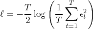
The conditional sum of squares function does not require the normality assumption. The initial observations , and , are set to zero.

Let be an ARFIMA() process represented as

then the conditional sum of squares function is