| Language Reference |
ARMACOV Call
computes an autocovariance sequence for an ARMA model
- CALL ARMACOV( auto, cross, convol, phi, theta, num);
The inputs to the ARMACOV subroutine are as follows:
- phi
- refers to a
 matrix
containing the autoregressive parameters.
The first element is assumed to have the value 1.
matrix
containing the autoregressive parameters.
The first element is assumed to have the value 1.
- theta
- refers to a
 matrix
containing the moving-average parameters.
The first element is assumed to have the value 1.
matrix
containing the moving-average parameters.
The first element is assumed to have the value 1.
- num
- refers to a scalar containing
 , the number of
autocovariances to be computed, which must be a positive number.
, the number of
autocovariances to be computed, which must be a positive number.
- auto
- specifies a variable to contain the returned
 matrix containing the autocovariances of the specified ARMA
model, assuming unit variance for the innovation sequence.
matrix containing the autocovariances of the specified ARMA
model, assuming unit variance for the innovation sequence.
- cross
- specifies a variable to contain the returned
matrix containing the covariances of the
moving-average term with lagged values of the process.
- convol
- specifies a variable to contain the returned
matrix containing the
autocovariance sequence of the moving-average term.
The model notation for the ARMACOV and ARMALIK subroutines is the same. The ARMA
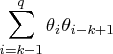
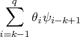
for
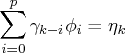
Consider the model
       /* an arma(1,1) model */
       phi  ={1 -0.5};
       theta={1 0.8};
       call armacov(auto,cross,convol,phi,theta,5);
       print auto,,cross convol;
The result is as follows:
                AUTO
           3.2533333 2.4266667 1.2133333 0.6066667 0.3033333


                     CROSS              CONVOL
                      2.04       0.8      1.64       0.8
Copyright © 2009 by SAS Institute Inc., Cary, NC, USA. All rights reserved.