Language Reference: MAD Function :: SAS/IML(R) 9.2 User's Guide

Language Reference

MAD Function

finds the univariate (scaled) median absolute deviation

MAD( ( $x\lt,spt\gt$ ))

where

x

is an

input data matrix.

spt

is an optional string argument with the following values:

"MAD": for computing the MAD (which is the default)
"NMAD": for computing the normalized version of MAD
"SN": for computing
"QN": for computing

The MAD function treats the input matrix

as univariate data by appending each row to the previous row to make a single row vector with elements $x_{11}, ... , x_{1p}, x_{21}, ... , x_{2p}, ... , x_{n1}, ... , x_{np}$ . In the following description, the notation

means the

th element of

when thought of as a row vector.

The MAD function can be used for computing one of the following three robust scale estimates:

median absolute deviation (MAD) or normalized form of MAD:
$mad_n = b * med_i^n \; | x_i - med_j^n \; x_j|$
where is the unscaled default and is used for the scaled version (consistency with the Gaussian distribution).
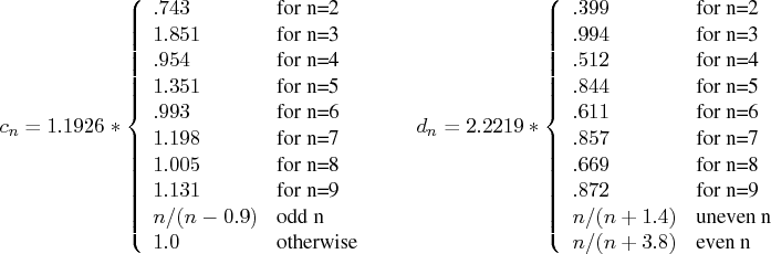
, which is a more efficient alternative to MAD:
$s_n = c_n * med_i \; med_{j \neq i} \; | x_i - x_j|$
where the outer median is a low median (order statistic of rank $[\frac{n+1}2]$ ) and the inner median is a high median (order statistic of rank $[\frac{n}2+1]$ ), and where is a scalar depending on sample size .
is another efficient alternative to MAD. It is based on the th-order statistic of the ${n \choose 2}$ inter-point distances:
$q_n = d_n * \{ | x_i - x_j|; i \lt j \}_{(k)} {with} k \approx {n \choose 2}/ 4$
where is a scalar similar to but different from . See Rousseeuw and Croux (1993) for more details.

The scalars

and

are defined as follows:

$c_n = 1.1926 * \{ .743 & {for n=2} \ 1.851 & {for n=3} \ .954 & {for n=4} \ ... ... .872 & {for n=9} \ n/(n + 1.4) & {uneven n} \ n/(n + 3.8) & {even n} .$

Example

The following example uses the univariate data set of Barnett and Lewis (1978). The data set is used in Chapter 9 to illustrate the univariate LMS and LTS estimates. Here is the code:

  
   b = { 3, 4, 7, 8, 10, 949, 951 }; 
  
   rmad1 = mad(b); 
   rmad2 = mad(b,"mad"); 
   rmad3 = mad(b,"nmad"); 
   rmad4 = mad(b,"sn"); 
   rmad5 = mad(b,"qn"); 
   print "Default MAD=" rmad1, 
         "Common MAD =" rmad2, 
         "MAD*1.4826 =" rmad3, 
         "Robust S_n =" rmad4, 
         "Robust Q_n =" rmad5;

This program produces the following output:

  
              Default MAD=         4 
              Common MAD =         4 
              MAD*1.4826 = 5.9304089 
              Robust S_n =  7.143674 
              Robust Q_n = 5.7125049

Top of Page