| Language Reference |
LCP Call
solves the linear complementarity problem
- CALL LCP( rc,
 ,
,  ,
,  ,
,  , epsilon>
);
, epsilon>
);
The inputs to the LCP subroutine are as follows:
- is an
 matrix.

- is an
 matrix.
- epsilon
- is a scalar defining virtual zero.
The default value of epsilon is 1.0E-8.
- rc
- returns one of the following scalar return codes:
- 0
- solution found
- 1
- no solution possible
- 5
- solution is numerically unstable
- 6
- subroutine could not obtain enough memory
- and
- return the solution in an -element column vector.
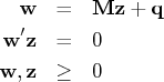
The LCP subroutine solves the linear complementarity problem:

    q={1, 1};
    m={1 0,
       0 1};
   call lcp(rc,w,z,m,q);
The result is as follows:
          RC            1 row       1 col     (numeric)

                                    0


          W             2 rows      1 col     (numeric)

                                    1
                                    1


          Z             2 rows      1 col     (numeric)

                                    0
                                    0
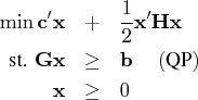
The next example shows the relationship between quadratic
programming and the linear complementarity problem.
Consider the linearly constrained quadratic program:
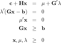
![m & = & [ h & -g^' \ g & 0 \ ] \ w^' & = & ({\mu }^'s^') \ z^' & = & (x^'{\lambda}^') \ q^' & = & (c^' - b)](images/langref_langrefeq676.gif)
![c^' & = & (1 2 4 5) b^' = ( 1 1 ) \ h & = & [ 100 & 10 & 1 & 0 \ 10 & 100 ... ... 0 & 1 & 10 & 100 ] \ g & = & [ 1 & 2 & 3 & 4 \ 10 & 20 & 30 & 40 ] \](images/langref_langrefeq683.gif)
       /*---- Data for the Quadratic Program -----*/
    c={1,2,3,4};
    h={100 10 1 0, 10 100 10 1, 1 10 100 10, 0 1 10 100};
    g={1 2 3 4, 10 20 30 40};
    b={1, 1};

       /*----- Express the Kuhn-Tucker Conditions as an LCP ----*/
    m=h||-g`;
    m=m//(g||j(nrow(g),nrow(g),0));
    q=c//-b ;

       /*----- Solve for a Kuhn-Tucker Point --------*/
    call lcp(rc,w,z,m,q);

       /*------ Extract the Solution to the Quadratic Program ----*/
    x=z[1:nrow(h)];
    print rc x;
The printed solution is as follows:
                 RC            1 row       1 col     (numeric)

                                           0

                 X             4 rows      1 col     (numeric)

                                   0.0307522
                                   0.0619692
                                   0.0929721
                                   0.1415983
Copyright © 2009 by SAS Institute Inc., Cary, NC, USA. All rights reserved.