Graphics Examples

Coordinate Systems

Each IML graph is associated with two independent cartesian coordinate systems, a world coordinate system and a normalized coordinate system.

Understanding World Coordinates

The world coordinate system is the coordinate system defined by your data. Because these coordinates help define objects in the data's two-dimensional world, these are referred to as world coordinates. For example, suppose that you have a data set containing heights and weights and that you are interested in plotting height versus weight. Your data induces a world coordinate system in which each point represents a pair of data values (height,weight). The world could be defined by the observed ranges of heights and weights, or it could be enlarged to include a range of all reasonable values for heights and weights.

Now consider a more realistic example of the stock price data for ACME Corporation. Suppose that the stock price data were actually the year-end prices of ACME stock for the years 1971 through 1986, as follows:

  
            YEAR   PRICE 
              71   123.75 
              72   128.00 
              73   139.75 
              74   155.50 
              75   139.75 
              76   151.50 
              77   150.375 
              78   149.125 
              79   159.50 
              80   152.375 
              81   147.00 
              82   134.125 
              83   138.75 
              84   123.625 
              85   127.125 
              86   125.500
 

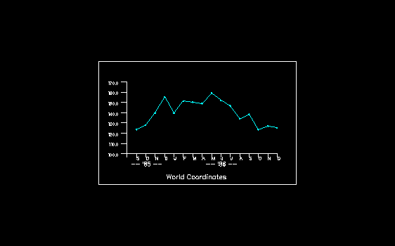
The actual range of YEAR is from 71 to 86, and the range of PRICE is from $123.625 to $159.50. These are the ranges in world coordinate space for the stock data. Of course, you could say that the range for PRICE could start at $0 and range upwards to, for example, $200. Or, if you were interested only in prices during the 80s, you could say the range for PRICE is from $123.625 to $152.375. As you see, it all depends on how you want to define your world.

Figure 12.2 shows a graph of the stock data with the world defined as the actual data given. The corners of the rectangle give the actual boundaries for this data.

Figure 12.2: World Coordinates

Understanding Normalized Coordinates

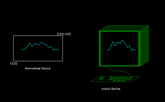
The normalized coordinate system is defined relative to your display device, usually a monitor or plotter. It is always defined with points varying between (0,0) and (100,100), where (0,0) refers to the lower-left corner and (100,100) refers to the upper-right corner.

In summary,

• the world coordinate system is defined relative to your data
• the normalized coordinate system is defined relative to the display device

Figure 12.3 shows the ACME stock data in terms of normalized coordinates. There is a natural mathematical relationship between each point in world and normalized coordinates. The normalized device coordinate system is mapped to the device display area so that (0,0), the lower-left corner, corresponds to (71, 123.625) in world coordinates, and (100,100), the upper-right corner, corresponds to (86,159.5) in world coordinates.

Figure 12.3: Normalized Coordinates