Model Fitting: Robust Regression
Frequently, robust regression is used to identify outliers and leverage points.
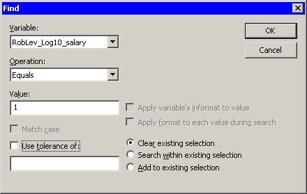
You can easily select outliers and leverage points by using the mouse to select observations in the RD plot, or by using the
Find dialog box. (You can display the Find dialog box by selecting → from the main menu.) The analysis added two indicator variables to the data table. The variable RobLev_Log10_salary has the value 1 for observations that are high leverage points. The variable RobOut_Log10_salary has the value 1 for the single observations that is an outlier.
Figure 22.7 shows how you can select all of the leverage points. After the observations are selected, you can examine their values, exclude them, change the shapes of their markers, or otherwise give them special treatment.
Similarly, you can select outliers.
To indicate a typical analysis of data that are contaminated with outliers:
-
Examine the outliers.
-
If it makes sense to exclude the observation from future analyses, select → → from the main menu.
-
Use ordinary least squares regression to model the data without the presence of outliers.
Note: You can select on the Tables tab. The parameter estimates in this table are the ordinary least squares estimates after excluding outliers.
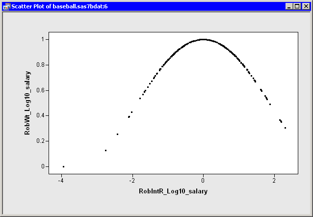
A second approach involves using the "Final Weights" variable that you requested on the Output Variables tab. The MM method uses an iteratively reweighted least squares algorithm to compute the final estimate, and the RobWt_Log10_salary variable contains the final weights.
Figure 22.8 shows the relationship between the weights and the studentized residuals. The graph shows that observations with large residuals
(in absolute value) receive little or no weight during the reweighted least squares algorithm. In particular, Steve Sax receives
no weight, and so his salary was not used in computing the final estimate. For this example, Tukey’s bisquare function was
used for the ![]() function in the MM method; if you use the Yohai function instead, Figure 22.8 looks different.
function in the MM method; if you use the Yohai function instead, Figure 22.8 looks different.
You can use the final weights to duplicate the parameter estimates by using ordinary least squares regression. For example,
if you run the REG procedure on the Baseball data and use RobWt_Log10_salary as a WEIGHT variable, you get approximately the same parameter estimates table as displayed by the ROBUSTREG procedure: