In the previous example you created a rotating scatter plot. A rotating scatter plot does not presume any relationship between the Z variable and the X and Y variables.

In this section you create a rotating plot in which you assume that the Z variable is functionally related to the X and Y variables. That is, the Z variable can be modeled as a response variable of X and Y.

A typical use of the rotating surface plot is to visualize the response surface for a regression model of two continuous variables. If you model a response variable by using an analysis chosen from the Analysis Model Fitting menu, you can add the predicted values of the model to the data table. Then you can plot the predicted values as a function of the two regressor variables.

In this example you examine three variables in the Climate data set. You explore the functional relationship between the elevationFeet variable and the latitude and longitude variables. The elevationFeet variable gives the elevation in feet above mean sea level for each of 40 cities in the continental United States.

To create a rotating plot and add a surface:

1. Open the Climate data set.

2. Select Graph Rotating Plot from the main menu.

   The Rotating Plot dialog box appears. (See Figure 7.9.)

3. Select the elevationFeet variable, and click Set Z.

4. Select the latitude variable, and click Set Y.

5. Select the longitude variable, and click Set X.

6. Click OK.

   Figure 7.9 The Rotating Plot Dialog Box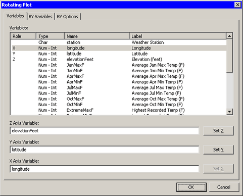

   
   
   

   A rotating plot appears (Figure 7.10), which shows a cloud of points. You can rotate the plot as explained in the previous example.

   Figure 7.10 A Rotating Plot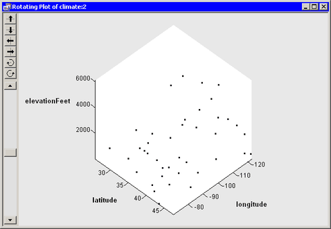

   
   
   

   You can visualize elevation as a function over longitude and latitude by adding a surface to these data.

7. Right-click near the center of the plot, and select Plot Area Properties from the pop-up menu.

8. Select Smooth color mesh from the group of radio buttons labeled Surface drawing modes.

9. Click OK.

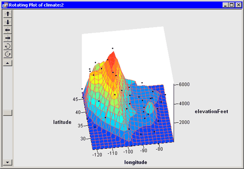
   The rotating plot updates to show a rough approximation to an elevation map of the continental United States. (See Figure 7.11.) There are only 40 data points in the plot, so the surface map is understandably coarse. Having more data points distributed uniformly across the country would result in a surface that is a better approximation of actual elevations.

   Nevertheless, the surface helps you to identify cities near the Rocky Mountains with high elevations (Cheyenne, WY, and Albuquerque, NM), one city in the Appalachian Mountains (Asheville, NC), and the coastal cities.

Figure 7.11 A Rotating Plot

Note:You can add a surface to any rotating scatter plot, but you should first determine whether it is appropriate to do so. Surface plots might not be appropriate for data with replicated measurements. Surface plots of highly correlated data can be degenerate.