| Distribution Analysis: Outlier Detection |
Example: Detect Univariate Outliers
In this example, you detect outliers for the pressure_outer_isobar variable of the Hurricanes data set. The Hurricanes data set contains 6,188 observations of tropical cyclones in the Atlantic basin. The pressure_outer_isobar variable gives the sea-level atmospheric pressure for the outermost closed isobar of a cyclone. This is a measure of the atmospheric pressure at the outermost edge of the storm. There are 4,662 nonmissing values of pressure_outer_isobar.
To find outliers in univariate data:
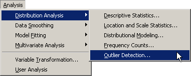
Select Analysis  Distribution Analysis Outlier Detection from the main menu, as shown in Figure 17.1.
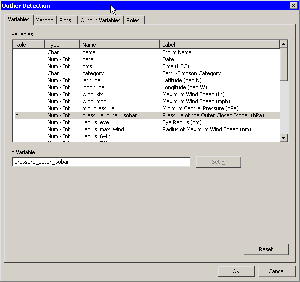
The Outlier Detection dialog box appears. (See Figure 17.2.) You can select a variable for the analysis by using the Variables tab.
Select the variable pressure_outer_isobar, and click Set Y.
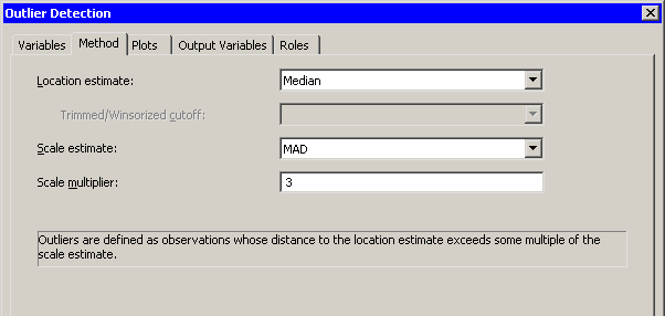
You can specify how the location and scale parameters are estimated by using the Method tab.
Click the Method tab.
The Method tab becomes active. (See Figure 17.3.) The default is to estimate the location with the median of the data, and to estimate the scale with the median absolute deviation from the median (MAD). Each estimate is described in the documentation for the UNIVARIATE procedure in the Base SAS Procedures Guide. The default scale multiplier is 3.
You can accept the default method parameters for this example.
Click the Plots tab.
The Plots tab becomes active. (See Figure 17.4.)
Select Normal quantile-quantile plot.
Click OK.
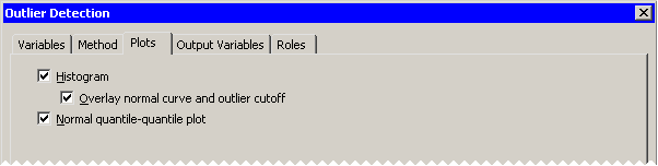
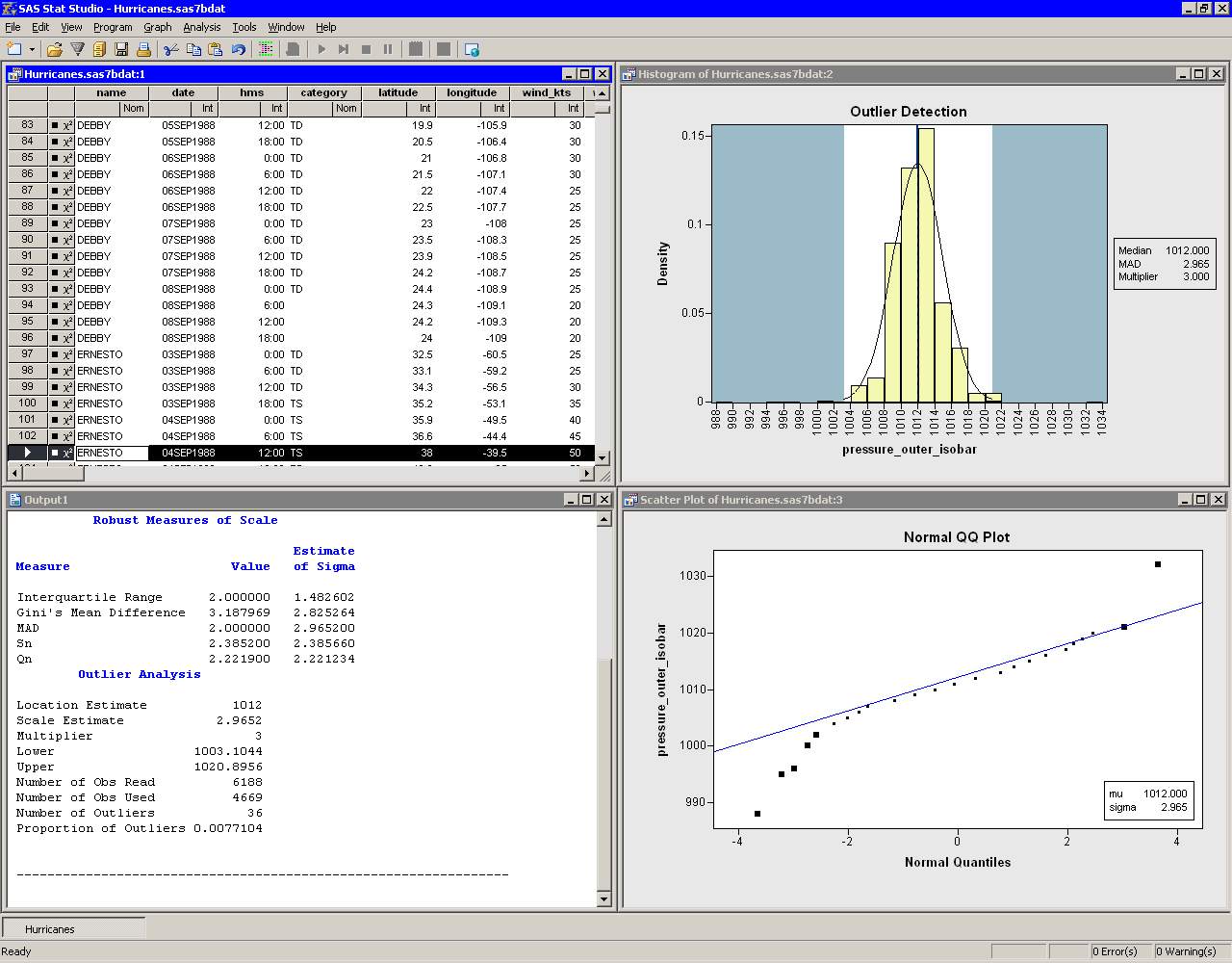
Figure 17.5 shows the results of this analysis. The analysis calls the UNIVARIATE procedure, which uses the options specified in the dialog box. The procedure displays tables in the output document. The tables show several estimates of the location and scale parameters. For this example, the median is 1012 hPa with a scale estimate of 2.965. SAS/IML statements are then used to read in the specified estimates and to compute values of pressure_outer_isobar that are more than  units away from 1012.
Two plots are created. One shows a histogram of the selected variable. The histogram is overlaid with a normal curve with  and
and  . A vertical line at 1012 indicates the location estimate, and shading indicates regions that are more than 8.965 units from 1012. The other plot is a normal Q-Q plot of the data.
By default, the analysis adds an indicator variable to the data table. The indicator variable is named Outlier_Y, where Y is the name of the chosen variable. You can select all observations that are marked as outliers by doing the following:
Select the data table window to make it active.
Select Edit Find from the main menu.
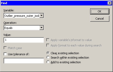
The Find dialog box appears as in Figure 17.6.
Select Outlier_pressure_outer_isobar from the Variable list.
Select Equals from the Operation list.
Type 1 in the Value box.
Click OK.
There are 36 observations marked as outliers. If the data table is active, you can use the F3 key to advance to the next selected observation. (Alternatively, you can use Edit Observations Examine Selected Observations to examine each selected observation in turn.) The normal Q-Q plot shows that the quantiles of the unselected observations fall along a straight line, which indicates that those observations appear to be normally distributed. (See Figure 17.5.) The selected observations (the outliers) deviate from the line.
Copyright © SAS Institute, Inc. All Rights Reserved.