| Distribution Analysis: Location and Scale Statistics |
Example: Compute Location and Scale Statistics
In this example, you compute statistics that estimate the location and scale for the pressure_outer_isobar variable of the Hurricanes data set. The Hurricanes data set contains 6,188 observations of tropical cyclones in the Atlantic basin. The pressure_outer_isobar variable gives the sea-level atmospheric pressure for the outermost closed isobar of a cyclone. This is a measure of the atmospheric pressure at the outermost edge of the storm. The pressure_outer_isobar variable contains 4,669 nonmissing values.
To compute estimates for the location and scale parameters:
Create a histogram of the pressure_outer_isobar variable.
A histogram appears, as shown in Figure 14.1.
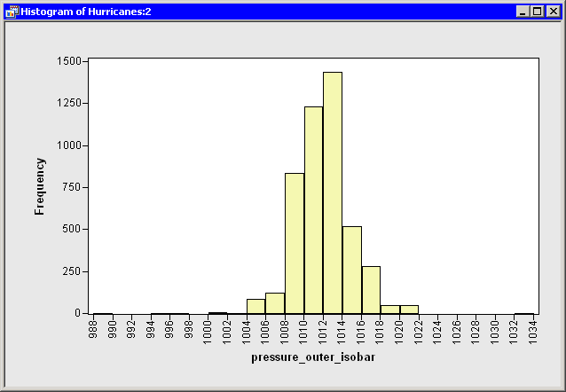
The histogram indicates that there are outliers in these data. Consequently, you might decide to compute robust estimates of location and scale for this variable, in addition to traditional estimates.
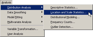
Select Analysis  Distribution Analysis Location and Scale Statistics from the main menu, as shown in Figure 14.2.
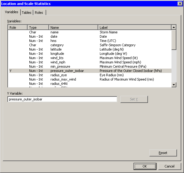
The Location and Scale Statistics dialog box appears. (See Figure 14.3.) You can select a variable for the univariate analysis on the Variables tab.
Select the variable pressure_outer_isobar, and click Set Y.
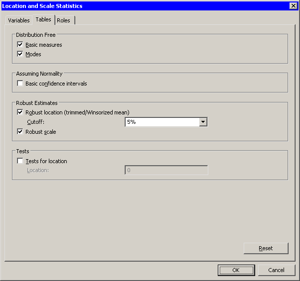
Click the Tables tab.
The Tables tab becomes active. (See Figure 14.4.)
Select Modes.
The following steps compute robust estimates for the location and scale of these data:
Select Robust location (trimmed/Winsorized mean).
Select Robust scale.
Click OK.
The analysis calls the UNIVARIATE procedure, which uses the options specified in the dialog box. The procedure displays tables in the output document, as shown in Figure 14.5.
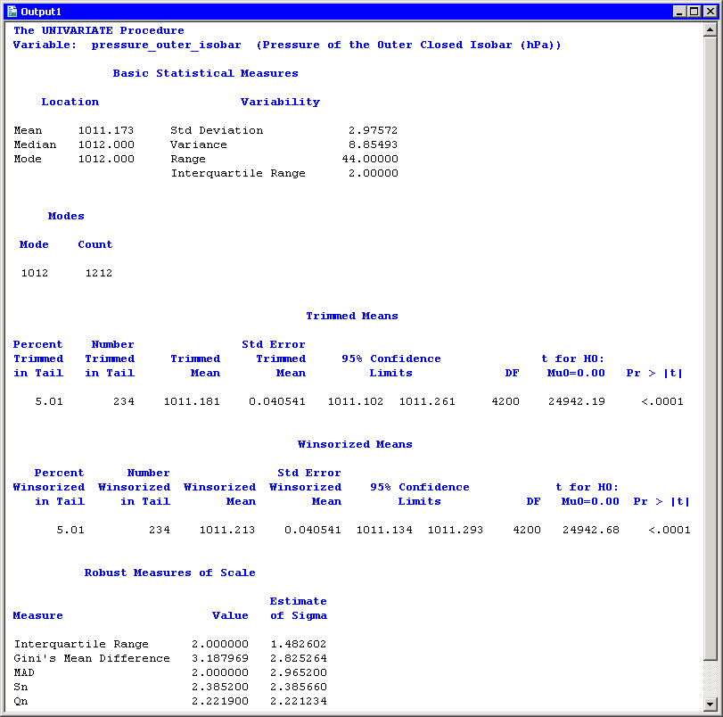
For the pressure_outer_isobar variable, the location statistics are in the range of 1011–1012 hPa. Most of the scale statistics are in the range of 2–3 hPa.
The mean is a nonrobust statistic, whereas the median, trimmed mean, and Winsorized mean are robust. Note that there is not much difference between the nonrobust and robust statistics of location for these data. The pressure_outer_isobar variable has outliers with extreme high and extreme low values. Therefore, the outliers did not appreciably change the mean. In general, the mean is affected by outliers.
Robust statistics of scale are listed in the "Robust Measures of Scale" table (not shown in Figure 14.5). The table has two columns. The first column lists the value of each robust statistic, and the second column scales the statistics to estimate the normal standard deviation under the assumption that the data are from a normal sample. The "Details" section of the UNIVARIATE procedure documentation presents details about the statistics in this table.
The values of the interquartile range and the MAD statistics should be interpreted with caution for these data because the values of the pressure_outer_isobar variable are discrete integers. More important, meteorologists traditionally display on weather maps only the isobars that correspond to even values. For these data, more than 81% of the nonmissing data are even integers.
Copyright © SAS Institute, Inc. All Rights Reserved.