Distribution Analysis: Distributional Modeling

Example

In this example, you fit a normal distribution to the pressure_outer_isobar variable of the Hurricanes data set. The Hurricanes data set contains 6188 observations of tropical cyclones in the Atlantic basin. The pressure_outer_isobar variable gives the sea-level atmospheric pressure for the outermost closed isobar of a cyclone. This is a measure of the atmospheric pressure at the outermost edge of the storm.

The plots and statistics in the Distributional Modeling analysis can help you answer questions such as the following:

Can these data be modeled by a parametric distribution? For example, are the data normally distributed?
If not, which characteristics of the data depart from the fitted distribution? For example, is the data distribution long-tailed? Is it skewed?
What proportion of the data is within a given range of values?

Answers to these questions for the pressure_outer_isobar variable appear at the end of this example.

Open the Hurricanes data set.

Create a histogram of the pressure_outer_isobar variable.

A histogram appears, as shown in Figure 15.1.

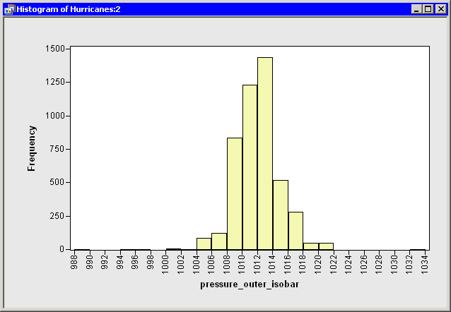Figure 15.1: A Histogram

From the shape of the histogram, you might wonder if the data distribution can be modeled by a normal distribution. If not, how do these data deviate from normality? The following steps add a normal curve to the histogram, and create other plots and statistics.

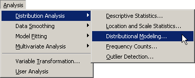Select Analysis $\blacktriangleright\,$ Distribution Analysis $\blacktriangleright\,$ Distributional Modeling from the main menu, as shown in Figure 15.2.

Figure 15.2: Selecting the Distributional Modeling Analysis

A dialog box appears as in Figure 15.3. You can select a variable for the univariate analysis by using the Variables tab.

Select the variable pressure_outer_isobar, and click Set Y.

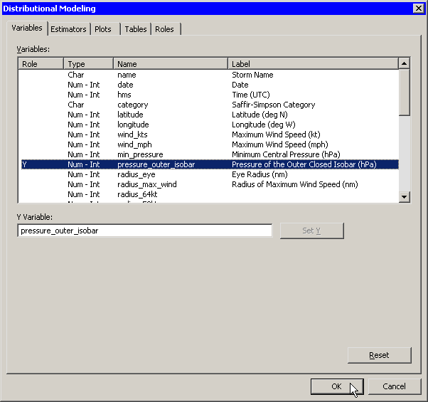Figure 15.3: Selecting a Variable

Click the Estimators tab.

The Estimators tab is shown in Figure 15.4.

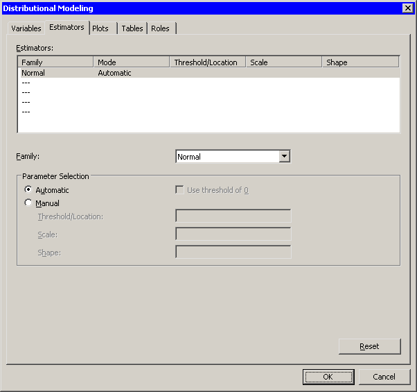ugdistmodelestimatorstab.png (9132 bytes)

Figure 15.4: Selecting a Distribution Family

The Estimators tab enables you to select distributions to fit to the data. For each distribution, you can enter known parameters, or indicate that the parameters should be estimated by maximum likelihood.

The section "Specifying Multiple Density Curves" describes how to create a histogram overlaid with more than one density curve. For this example, you select a single distribution to fit to the data.

The normal distribution appears in the Estimators list by default. Also by default, the Automatic radio button is selected. This specifies that the location and scale parameters for the normal distribution be determined by using maximum likelihood estimation.

Accept these defaults and proceed to the next tab.

Click the Plots tab.

Select all plots, as shown in Figure 15.5.

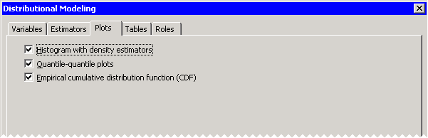Figure 15.5: Selecting Plots

Click OK.

The analysis calls the UNIVARIATE procedure, which uses the options specified in the dialog box. The procedure displays tables in the output document, as shown in Figure 15.6.

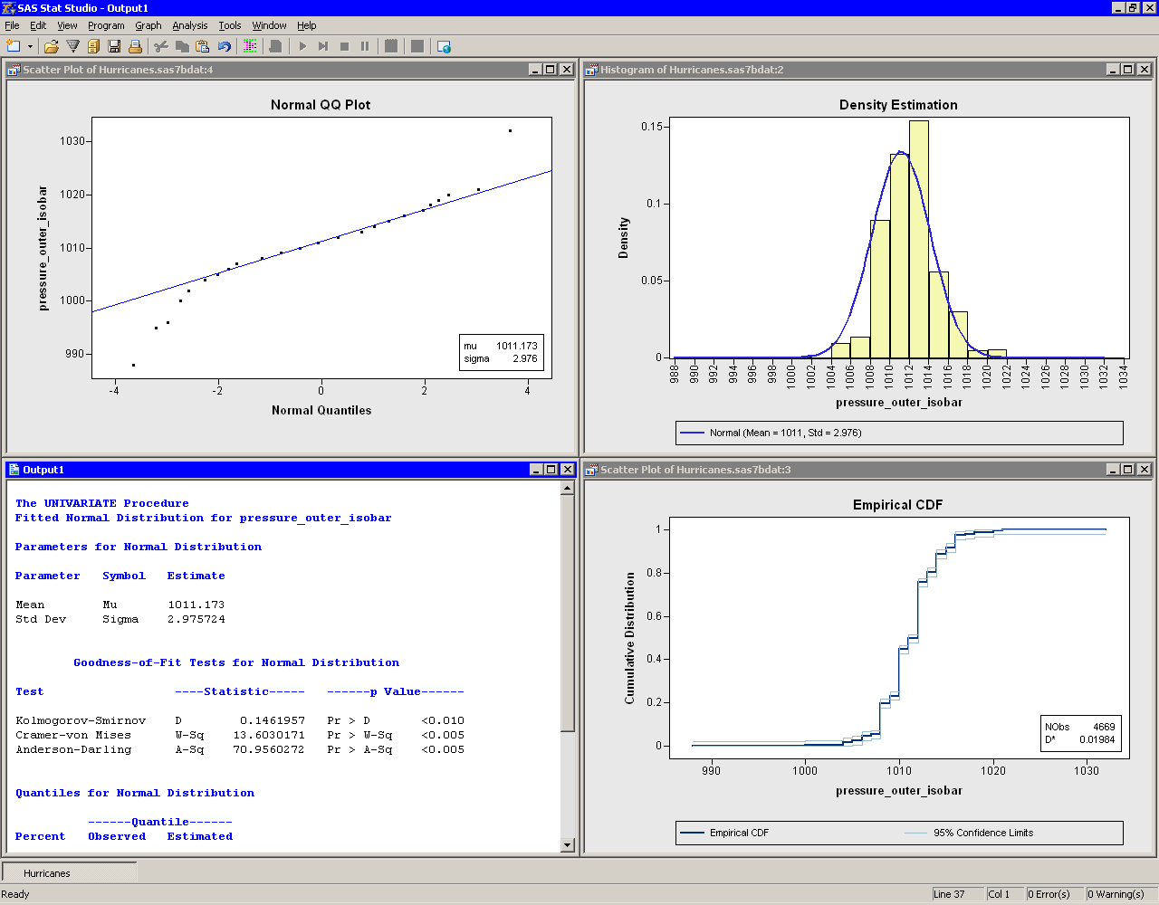Figure 15.6: Output from a Distributional Modeling Analysis

Several plots are created. These plots can help answer the questions posed earlier.

Are the Data Normal?

The histogram (the upper-right plot in Figure 15.6) is overlaid with a normal density curve. The curve does not fit the data in several locations. The curve predicts more observations in the [1006, 1008] bin than actually occur, and underestimates the count in the [1012, 1014] bin.

How Do the Data Deviate from Normality?

A normal Q-Q plot appears as the upper-left plot in Figure 15.6. A Q-Q plot graphically indicates whether there is agreement between quantiles of the data and quantiles of a theoretical distribution. The Q-Q plot for the normal distribution shows several points to the left that are below the diagonal line. These points indicate that the data distribution has a longer left tail than would be expected from normally distributed data. The point to the right that is above the line might indicate an outlier in the data. Table 15.1 describes how to interpret common features of a Q-Q plot.

The goodness-of-fit table in the output document shows that the -values for the goodness-of-fit tests are very small. The null hypothesis for the goodness-of-fit tests is that the data are from a specified theoretical distribution. The smaller the -value, the stronger the evidence against the null hypothesis. The small -values in this example indicate that the normal distribution is not an adequate model to describe these data.

Note: The pressure_outer_isobar variable contains 4669 nonmissing values. For a sample of this size, the goodness-of-fit tests can detect small departures from normality, so it is not surprising that these tests reject the null hypothesis.

What Proportion of the Data Satisfies Certain Conditions?

A CDF plot appears as the lower-right plot in Figure 15.6. The CDF plot shows a graph of the empirical cumulative distribution function. You can use the CDF plot to examine relationships between data values and data proportions.

For example, Figure 15.7 graphically answers the question, What observations are contained in the upper quintile (20%) of the data? The selected observations answer the question: data values greater than or equal to 1013 hPa. Similarly, you can ask a converse question: What percentage of the data has values less than or equal to 1000 hPa? The answer (0.4%) can also be obtained by interacting with the CDF plot.

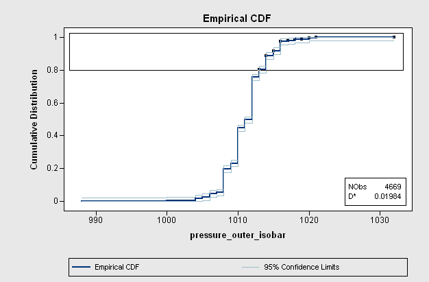Figure 15.7: A CDF Plot

The CDF plot also shows how data are distributed. For example, the long vertical jumps in the CDF that occur at even values (1008, 1010, and 1012 hPa) indicate that there are many observations with these values. In contrast, the short vertical jumps at odd values (for example, 1009, 1011, and 1013 hPa) indicate that there are not many observations with these values. This fact is not apparent from the histogram, because the default bin width is 2 hPa.

Top of Page