Common Tasks
The following sections show the coding that is necessary
to accomplish several common tasks for managing ODS graphics output.
Controlling the Image Name and Image Format
Specifying the Image Name
For
ODS Graphics output, by default, the ODS object name is used as the
“root” name for the image output file.
The following example
creates a GIF image named REGPLOT:
ods graphics / imagename="regplot" outputfmt=gif;
The assigned name REGPLOT
is treated as a "root" name and the first output created is named
REGPLOT. Subsequent graphs are named REGPLOT1, REGPLOT2, and so on,
with an increasing index counter. All graphs in this example will
be GIF images.
If you are developing
a template and its takes several submissions to get the desired output,
you might want to use the RESET or RESET= option to force each output
to replace itself:
ods graphics / reset=index ... ;This specification causes all subsequent images to be created with the default or current image name.
Specifying the Image Format
Each ODS destination uses a default image format for
its output. Depending on the destination, the image output format
is Portable Network Graphics (PNG) or vector graphics. See SAS Output Delivery System: User's Guide for more information. You can use the OUTPUTFMT=
option in the ODS GRAPHICS statement to change the output format.
Unless you have a special
requirement for changing the image format, we recommend that you not
change it. The default PNG or vector graphic format is far superior
to other formats, such as GIF, in support for transparency and a large
number of colors. Also, PNG and vector graphics images require much
less disk storage space than JPEG or TIFF formats. Additional advantages
that are provided by vector graphics images include scalability and
multiple output formats, which are PDF, EMF, and SVG.
If you want to generate vector graphics images, you can use the ODS
destination and ODS GRAPHICS statement OUTPUTFMT= option combinations
that are shown in Generating Vector Graphics Images with ODS.
If a vector graphics
image cannot be generated for the image format that you specify, a
PNG image is generated instead and is embedded in the specified output
file. The output file format and extension are not changed in that
case. Cases where a vector graphics image cannot be generated include
the following:
Controlling the Image's Output Location
To control the image
location (path) for ODS Graphics output, use the PATH= or GPATH=
option on the ODS destination statement.
ods listing gpath="C:\ODSgraphs";

ods html gpath="C:\ODSgraphs";
For the HTML destination,
the PATH= option is used to indicate whether the HTML page is stored.
If GPATH= is not used, images are stored at the PATH= storage location.
Use PATH= and GPATH= together when you want to store images in a different
storage location. The (URL= NONE | url-spec) suboption specifies a Uniform Resource Locator for the PATH= or
the GPATH= options.
ods graphics / reset imagename="graph";
ods html style=statistical
         path="u:\public_html"
         gpath="u:\public_html" (url=none)
         file="report.html";

proc sgrender data=sashelp.heart template=modelfit
              des="Regression Fit plot";
run;
proc sgrender data=sashelp.heart template=distribution
              des="Distribution of Cholesterol";
   dynamic var="Cholesterol";
run;
ods html close;
ods html;
The graphs produced
are named graph.png and graph1.png and are stored in u:\public_html\.
The (URL=NONE) suboption prevents any path or URL information from
being included in the SRC=" " attribute of the <IMG> tag. This
creates relative references to the images in the html source:
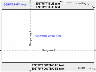
Controlling Graph Size
BEGINGRAPH Statement
When creating a graphics
template, you often want to control the design width and design height,
especially for multi-cell graphs.
BEGINGRAPH / DESIGNWIDTH= dimension DESIGNHEIGHT= dimension;
In addition to specifying sizes in several units, you
can also refer to the current registry settings with the constants
DEFAULTDESIGNWIDTH and DEFAULTDESIGNHEIGHT.
In the following example,
the intent is to produce a square graph (equal height and width) in
order to reduce unused graphical area. The design width is set to
the default internal height (DEFAULTDESIGNHEIGHT).
proc template;
  define statgraph squareplot;
    dynamic title xvar yvar;
    begingraph / designwidth=defaultDesignHeight;
      entrytitle title;
      layout overlayequated / equatetype=square;
         scatterplot x=xvar y=yvar;
         regressionplot x=xvar y=yvar;
      endlayout;
    endgraph;
  end;
run;
If this template were
executed with the following SGRENDER specification, a 480px by 480px
graph would be created:
proc sgrender data=mydata template="squareplot";
  dynamic title="Square Plot" xvar="time1" yvar="time2";
run;
If a 550px width or
height were set on an ODS GRAPHICS statement before the template is
executed with the SGRENDER procedure, a 550px by 550px graph would
be created, maintaining the 1:1 aspect ratio:
ods graphics / width=550px;
proc sgrender data=mydata template="squareplot";
  dynamic title="Square Plot" xvar="time1" yvar="time2";
run;

/* Setting a 550px height would create the same size graph */
ods graphics / height=550px;
proc sgrender data=mydata template="squareplot";
  dynamic title="Square Plot" xvar="time1" yvar="time2";
run;
When no DESIGNWIDTH= or DESIGNHEIGHT= option is specified in the
BEGINGRAPH statement, graphs are rendered with the registry defaults,
unless changed by the ODS GRAPHICS statement HEIGHT= or WIDTH= options.
Examples for sizing
multi-cell graphs are discussed in Using a Simple Multi-cell Layout, Using an Advanced Multi-cell Layout, and Using Classification Panels.
Understanding Graph Scaling
ODS graphics uses style information to control the appearance
of the graph. Style definitions contain information about fonts, color,
lines, and markers, and they also contain settings such as font size
and marker size. When a graph is rendered at a size larger or smaller
than its design size, scaling takes place by default.
ods graphics / width=480px height=360px scale=on ;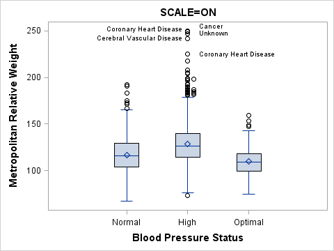
If you turn off scaling, the font sizes,
marker sizes, and so on, revert to the sizes that are defined in the
style. To accommodate the larger font sizes for the titles, footnotes,
axis labels, tick values, and data labels, the wall area and contained
graphical components automatically shrink.
ods graphics / width=480px height=360px scale=off ;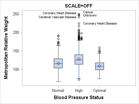
In general, having the
fonts scale up or down as the graph size increases or decreases is
desirable. However, in some cases you might want greater control of
the font sizes.
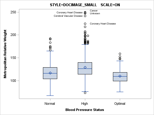
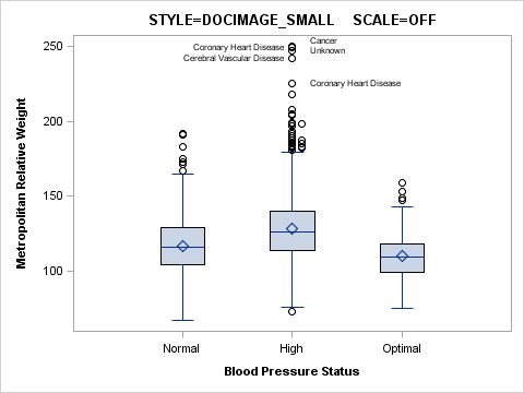
The examples in this
document were created with different styles that varied only in the
font sizes that they used. In some cases, smaller graphs look better
when rendered in a smaller set of fonts. The style examples below
use the LISTING style as a parent, but you could use any style as
the parent. The DOCIMAGE style keeps fonts close to the default sizes
and weights, while the DOCIMAGE_SMALL style reduces the font sizes
by a few points. See Managing the Graph Appearance with Styles for a discussion
of defining you own styles and what parts of the graph are affected
by various style elements.
proc template;
  define style docimage;
    parent=styles.listing;
    style GraphFonts from GraphFonts
         "Fonts used in graph styles" /
         'GraphDataFont' = ("<sans-serif>, <MTsans-serif>",8pt)
         'GraphUnicodeFont' = ("<MTsans-serif-unicode>",10pt)
         'GraphValueFont' = ("<sans-serif>, <MTsans-serif>",10pt)
         'GraphLabelFont' = ("<sans-serif>, <MTsans-serif>",12pt,bold)
         'GraphFootnoteFont' = ("<sans-serif>, <MTsans-serif>",10pt)
         'GraphTitleFont' = ("<sans-serif>, <MTsans-serif>",12pt,bold);
  end;

  define style docimage_small;
    parent=styles.listing;
    style GraphFonts from GraphFonts
         "Fonts used in graph styles" /
         'GraphDataFont' = ("<sans-serif>, <MTsans-serif>",6pt)
         'GraphUnicodeFont' = ("<MTsans-serif-unicode>",8pt)
         'GraphValueFont' = ("<sans-serif>, <MTsans-serif>",8pt)
         'GraphLabelFont' = ("<sans-serif>, <MTsans-serif>",8pt,bold)
         'GraphFootnoteFont' = ("<sans-serif>, <MTsans-serif>",8pt)
         'GraphTitleFont' = ("<sans-serif>, <MTsans-serif>",10pt,bold);
  end;
run;
The previous two graphs
were created the DOCIMAGE style. These next two graphs were created
with the DOCIMAGE_SMALL style.
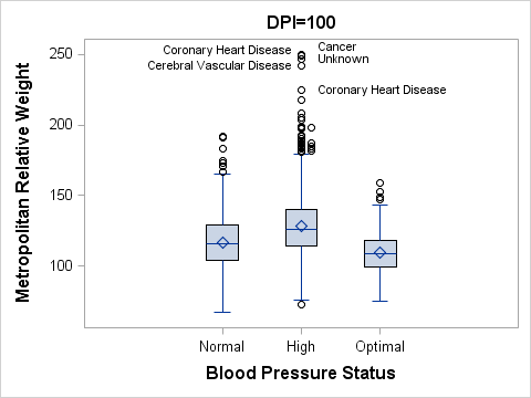
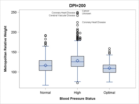
Controlling DPI
All ODS destinations
use a default DPI (dots per inch) setting when creating ODS Graphics
output. By default, LISTING and HTML use 100 dpi, while RTF and PDF
use 200 dpi. Graphs that are rendered at higher DPI have greater resolution
and larger file size. Although DPI can be set to large values such
as 1200, from a practical standpoint, settings larger than 300dpi
are seldom necessary for most applications. Also, setting an unrealistically
large DPI like 1200 could cause an out-of-memory condition. Note that
the ODS option for setting DPI is not the same for all destinations.
For the LISTING and HTML destinations, use the IMAGE_DPI= option.
For the RTF and PDF destinations, use the DPI= option.
ods graphics / width=480px height=360px scale=off;
ods html image_dpi=100 style=docimage_small;
Controlling Anti-Aliasing
Anti-aliasing is a graphical
rendering technique that improves the readability of text and the
crispness of the graphical primitives, such as the markers and lines.
By default, ODS Graphics uses anti-aliasing.
Note: Titles, footnotes, entry
text, axis labels, tick values, and legend text is always anti-aliased.
Graphical components related to the data, such as markers, lines,
and data labels, are affected by the ANTIALIAS= and ANTIALIASMAX=
options, as discussed in this section.
To see how much the
graph quality is improved with anti-aliasing, you can turn this feature
on and off with the ANTITALIAS= option in the ODS GRAPHICS statement.
ods graphics / antialias=on;
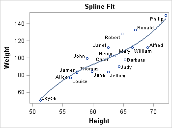
ods html image_dpi=100;
proc sgrender data=sashelp.class template=fitline;
run;
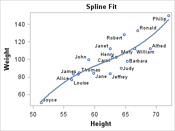
ods graphics / antialias=off ;
ods html image_dpi=100;
proc sgrender data=sashelp.class template=fitline;
run;
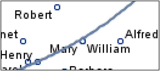
The following image
shows a zoomed-in view of a portion of the anti-aliased image (100dpi).
Notice that the text, markers, and line appear fuzzy because of the
anti-aliasing algorithm.
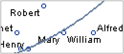
This next image shows
a zoomed-in view of the image (100dpi) that has anti-aliasing turned
off. Notice that the text, markers, and line are not fuzzy but have
a jagged appearance.
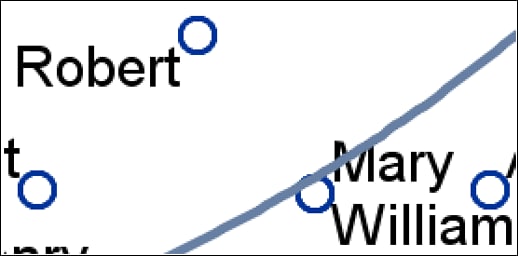
If the image is created
at 300dpi, the combination of anti-aliasing and higher resolution
produces a very high quality image.
To perform anti-aliasing
requires additional computer resources (CPU, memory, and execution
time). Graphs that have a lot of markers, lines, and text use even
more resources. Filled or gradient 3-D surface plots might require
even more resources.
Setting a higher DPI
increases anti-aliasing resources. At some point, ODS Graphics deems
that anti-aliasing requires too many resources and it turns the feature
off. When this happens, you will get a non-anti-aliased rendered graph
and a message in the SAS log similar to the following :
NOTE: Marker and line antialiasing has been disabled because the threshold has
      been reached. You can set ANTIALIASMAX=5700 in the ODS GRAPHICS
      statement to restore antialiasing.
Creating a Graph That Can Be Edited
SAS provides an application
called the ODS Graphics Editor that can be used to post-process ODS
Graphics output. With the editor, you can edit the following features
in a graph that was created using ODS Graphics:
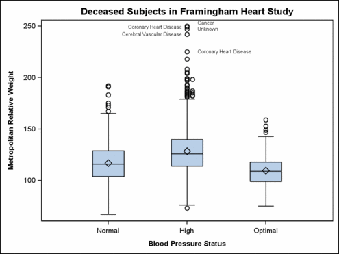
For example, suppose
the following template is used to create box plots in a graph and
you want to indicate that the labeled outliers are far outliers (more
than 3 IQR above 75th percentile).
proc template;
  define statgraph boxplot;
    begingraph;
      entrytitle "Deceased Subjects in Framingham Heart Study";
      layout overlay;
        boxplot y=mrw x=bp_status / datalabel=deathcause
                spread=true labelfar=true;
      endlayout;
    endgraph;
  end;
run;
To create ODS Graphics output that can be edited, you
must specify the SGE=ON option in the ODS LISTING destination statement
before creating the graph:
ods listing sge=on style=listing;

proc sgrender data=sashelp.heart template=boxplot;
  where status="Dead";
run;
When SGE=ON is in effect,
an .SGE file is created in addition to the image file normally produced.
From the Results Window, you can open the
.SGE file in the ODS Graphics Editor by selecting Open in the icon.
You can also open the .SGE file directly from the Windows file system.
The .SGE file is always created in the same location as the image
output. Here is the image output.
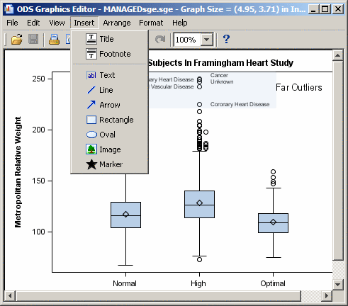
The following figure
shows the Graphical User Interface for the ODS Graphics Editor after
some of the annotation has been completed.
Creating a Graph to Include in MS Office Applications
The default height for
a graph is 480 pixels. At a 100 dot per inch (DPI) setting, you can
consider the default height to be 4.8 inches. If you render a graph
at 480 pixels and 100 DPI, insert it into a document like an MS Office
application, and then print the page, the graph height on paper will
be 4.8 inches and all font sizes will look right in their point weights.
You can render the graph at a higher DPI to get higher quality graphs.
As long as the graph is then inserted in the document as a 4.8 inch
graph, it will work as expected.
To alter the graph size or DPI
for a graph that you want to include in an MS Office application,
one technique that produces good results is to create a stand-alone
image that is sized appropriately and has high resolution, say 200
DPI or 300 DPI.
ods graphics / reset width=5in imagename="fitplot" outputfmt=png
    antialias=on;
ods listing gpath="\ODSgraphs" image_dpi=200 style=analysis;

proc sgrender data= . . . template= . . .;
run;
This code produces a
5 inch, 200 DPI image
\ODSgraphs\fitplot.png, which can be inserted into Word or PowerPoint documents. When only
the WIDTH= or HEIGHT= option is specified in the ODS GRAPHICS statement,
the design aspect ratio of the graph is maintained. Also, check the
SAS log to ensure that anti-aliasing has not been disabled. If it
has been disabled, add the ANTIALIASMAX= option (see Controlling Anti-Aliasing for a discussion
of anti-aliasing).
After inserting the
graph into the MS Office document, you can change the picture size
with good results (while maintaining aspect ratio). If you find that
the text in the graph is too large or too small, recreate the graph
with different font sizes using the techniques discussed in Understanding Graph Scaling.
To create good looking
graphs for a two-column MS Word document where each column is about
3.5 inches wide, use a graph width of 3.5 inches. If the original
graph has a default width of 640 pixels, you can set WIDTH=3.5IN in
the ODS GRAPHICS statement to get a smaller graph with appropriately
smaller fonts. In this case, the fonts will not be exactly the right
point size, but they will be scaled smaller using a non-linear scaling
factor.
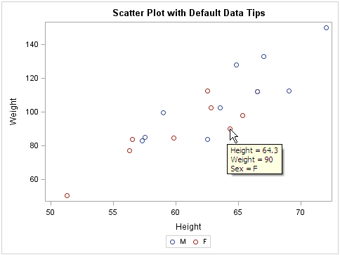
Controlling Data Tips
Creating a Graph with Data Tips in an HTML Page
Data tips (sometimes
called tooltips) can be displayed by graphs that are included in HTML
pages. When data tips are provided, you can "mouse over" parts of
a graph, and text balloons open to show information (typically data
values) that is associated with the area where the mouse pointer rests.
Nearly all plot statements in GTL create default data tip information.
However, this information is not generated unless you request it with
the IMAGEMAP= option in the ODS GRAPHICS statement:
ods html file=". . ." path=". . ." (url=none);
ods graphics / reset width=5in imagemap=on ;

proc sgrender data= . . . template= . . .;
run;

ods graphics / reset;
ods html close;
Creating a Graph with Custom Data Tips in an HTML Page
GTL supports plot statement
syntax that enables you to suppress or customize the default data
tip information. Here is an example:
layout overlay;
  /* scatter points have enhanced tooltips */
  scatterplot x=height y=weight / group=sex name="s"
    rolename=(tip1=name tip2=age)
    tip=(tip1 tip2 X Y GROUP)
    tiplabel=(tip1="Student Name")
    tipformat=(tip2=2.);
  discretelegend "s";
endlayout;
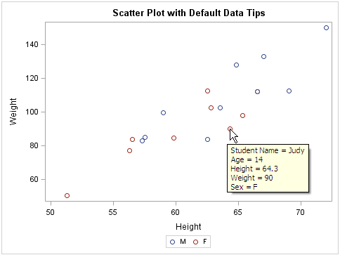
ROLENAME defines one
or more name / value pairs as role-name = column-name, where column-name is some input data column that does
not participate directly in the plot. In this example, we want the
NAME and AGE column values to show in the tip. Notice that the choice
of role names is somewhat arbitrary. The TIP1 and TIP2 role names
are added to the default role names X, Y, and GROUP.
The TIP= option defines
a list of roles to be displayed, and it also determines their order
in the display. Notice that it is not necessary to request all default
roles. For example, it might be obvious from the legend that the GROUP
role does not really need to be in the data tip, so in that case you
would specify:
tip=(tip1 tip2 X Y)