Features of Continuous Legends

Plots That Can Use Continuous Legends

A continuous legend maps the data range of a response variable to a range of colors. Continuous legends can be used with the following plot statements when the enabling plot option is also specified.

Plot Statement	Enabling Plot Option	Related Plot Options
CONTOURPLOTPARM	CONTOURTYPE=	COLORMODEL= REVERSECOLORMODEL= NLEVELS= NHINT=
HEATMAPPARM	COLORRESPONSE=	COLORMODEL=
SCATTERPLOT	MARKERCOLORGRADIENT=	COLORMODEL= REVERSECOLORMODEL=
SURFACEPLOTPARM	SURFACECOLORGRADENT=	COLORMODEL= REVERSECOLORMODEL=

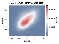
A contour plot provides the CONTOURTYPE= option, which you can use to manage the contour display. The following graph illustrates the values that are available for the CONTOURTYPE= option.

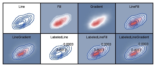
All of the variations that support color, except for LINE and LABELEDLINE, can have a legend that shows the value of the required Z= column. For example, the following code generates a contour plot with CONTOURTYPE=FILL:

proc template;
 define statgraph contour;
  begingraph;
   entrytitle "CONTOURTYPE=FILL";
   layout overlay / xaxisopts=(offsetmin=0 offsetmax=0)
                    yaxisopts=(offsetmin=0 offsetmax=0);
     contourplotparm x=Height y=Weight z=Density / name="cont"
       contourtype=fill ;
     continuouslegend "cont" / title="Density";
   endlayout;
  endgraph;
 end;
run;
 
proc sgrender data=sashelp.gridded template=contour;
 where height>=53 and weight<=225;
run;

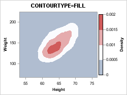
If you change to CONTOURTYPE=GRADIENT you get the following output:

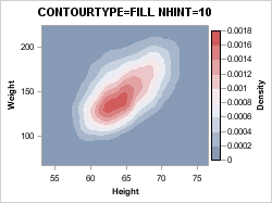
For a FILL contour, the Z variable is split into equal-sized value ranges, and each range is assigned a different color. The continuous legend shows the value range boundaries and the associated colors as a long strip of color swatches with an axis on it. The contour options NHINT= and NLEVELS= are used to change the number of levels (ranges) of the contour. NHINT=10 requests that a number near ten be used that results in "good" intervals for displaying in the legend. NLEVELS=10 forces ten levels to be used.

contourplotparm x=Height y=Weight
  z=Density / name="cont" 
  contourtype=fill nhint=10 ;
continuouslegend "cont" /
  title="Density";

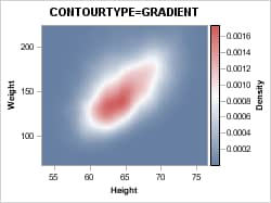
Legend Settings: COUNTOURTYPE-FILL, NHINT=10

You can think of a GRADIENT contour as a FILL contour with a very large number of levels. A color ramp is displayed with an axis that shows reference points that are within the data range. The number of reference points is determined by default.

When a CONTINUOUS legend is used with a plot that uses gradient color, the VALUESCOUNT= and VALUESCOUNTHINT= options can be used to manage the legend's gradient axis. These options are similar to the NLEVELS= and NHINT= plot options.

continuouslegend "cont" /
  title="Density"
  valuecounthint=5 ;

continuouslegend "cont" /
  title="Density"
  valuecounthint=10 ;

Positioning a Continuous Legend

The ACROSS= , DOWN=, and ORDER= options are not supported by the CONTINUOUSLEGEND statement. However, you can position a continuous legend with the LOCATION=, HALIGN=, VALIGN=, and ORIENT= options. By default, LOCATION=OUTSIDE and ORIENT=VERTICAL when HALIGN=RIGHT or HALIGN=LEFT.

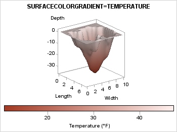
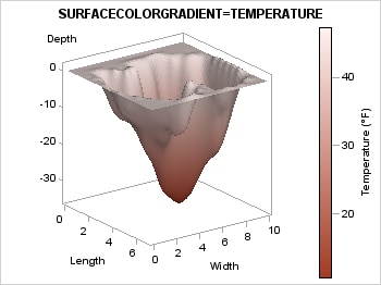
Using Color Gradients to Represent Response Values

Contour plots, surface plots, and heat map plots support the use of color gradients to represent response values. For example, the SURFACEPLOTPARM statement provides the SURFACECOLORGRADIENT=numeric-column setting to map surface colors to a continuous gradient and enable the use of a continuous legend. All surface types (FILL, FILLGRID, and WIREFRAME) can be used. The COLORMODEL= and REVERSECOLORMODEL= options also apply. For more information about surface plots, see Using 3-D Graphics.

ods escapechar="^"; /* Define an escape character */

proc template;
  define statgraph surfaceplot;
   begingraph;
    entrytitle "SURFACECOLORGRADIENT=TEMPERATURE";
    layout overlay3d / cube=false;
      surfaceplotparm x=length y=width z=depth / name="surf"
        surfacetype=fill
        surfacecolorgradient=temperature
        reversecolormodel=true
        colormodel=twocoloraltramp ;
      continuouslegend "surf" / 
        title="Temperature (^{unicode '00B0'x}F)"
        halign=right ;
    endlayout;
   endgraph;
  end;
run;
 
data lake;
  set sashelp.lake;
  if depth = 0 then Temperature=46;
  else Temperature=46+depth;
run;
 
/* create smoothed interpolated spline data for surface */	 
proc g3grid data=lake out=spline;
   grid width*length = depth temperature / naxis1=75 naxis2=75 spline;
run;

proc sgrender data=spline template=surfaceplot;
run;

When you use VALIGN=BOTTOM or VALIGN=TOP instead of the HALIGN= option , then the default orientation of the legend automatically becomes ORIENT=HORIZONTAL:

ods escapechar="^"; /* Define an escape character */
continuouslegend "surf" /
  title="Temperature (^{unicode '00B0'x}F)" 
  valign=bottom ;

Notice the coding that is used to embed a degree symbol into the legend title. For more information about using symbols in text, see Adding and Changing Text in a Graph.