Examples
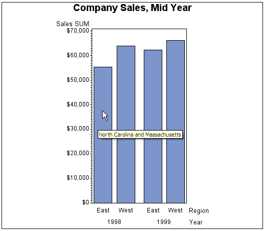
Example 1: Adding Custom Data Tips to a Graph in a Web Presentation
| Features: |
VBAR statement
|
| Other features: |
GOPTIONS statement option: BORDER |
Program
/* Create the temporary data set named sales. */
data sales;
   length Region $ 4 State $ 2;
   format Sales dollar8.;
   input Region State Sales Year Qtr;
   datalines;
West CA 13636 1999 1
West OR 18988 1999 1
West CA 14523 1999 2
West OR 18988 1999 2
East MA 18038 1999 1
East NC 13611 1999 1
East MA 11084 1999 2
East NC 19660 1999 2
West CA 12536 1998 1
West OR 17888 1998 1
West CA 15623 1998 2
West OR 17963 1998 2
East NC 17638 1998 1
East MA 12811 1998 1
East NC 12184 1998 2
East MA 12760 1998 2
;
/* Use an IF/THEN statement to assign values to the variable RPT. */
data sales;
   set sales;
      if state in ("NC" "MA") then
         RPT="title='North Carolina and Massachusetts'";
      if state in ("CA" "OR") then  RPT="title='California and Oregon'";
run;

/* Reset the graphics options to their defaults and specify a border. */
goptions reset=all border;

/* Close the current ODS HTML destination. */
ods html close;

/* Open the HTML destination and specify the ODS output filename */
/* and style.  */
ods html file="datatips.htm" style=listing;

/* Generate the bar chart. Add the HTML= option to associate */
/* the custom data tips with each graph element.             */
title "Company Sales, Mid Year";
proc gchart data=sales;
   vbar region / sumvar=sales
      group=year
      html=RPT;
run;
quit;

/* Close ODS HTML to close the output file, and then reopen it. */
ods html close;
ods html;
Example 2: Creating a Drill-Down HTML Presentation for the Web
| Features: |
VBAR statement
|
| Other features: |
AXIS statement BY statement FORMAT statement
LEGEND statement RUN-group processing TITLE statement WHERE statement |
| Sample library member: | GCHDDOWN |
About This Example
This example shows how
to create 2-D bar charts with drill-down functionality for the Web.
In addition to showing how to use the ODS HTML statement and the HTML
options to create the drill-down, the example also illustrates other
VBAR statement options.
For creating output
with drill-down functionality for the Web, the example shows how to
do the following tasks:
For more information,
see ODS HTML Statement.
The program generates
twelve linked bar charts that display data about the world's leading
grain producers. The charts are described in Output. The data contain
the amount of grain produced by five countries in 1995 and 1996. Each
of these countries is one of the three leading producers of wheat,
rice, or corn, worldwide.
Output
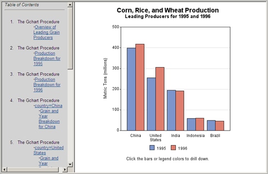
The first chart, shown
in Browser View of Overview Graph as it appears in a browser, is an overview of the data that shows
the total grain production for the five countries for both years.
Browser View of Overview Graph
The next two charts
break down grain production by year. These charts are linked
to the legend values in Browser View of Overview Graph. For example, when you
select the legend value for 1995, the graph in Browser View of Year Breakdown for 1995 appears.
Browser View of Year Breakdown for 1995
Another group
of charts breaks down the data by country. These charts are linked
to the bars in Browser View of Overview Graph and Browser View of Year Breakdown for 1995. For example,
when you click the bar for China in either Browser View of Overview Graph or Browser View of Year Breakdown for 1995, the
graph in Browser View of Breakdown for China appears.
Browser View of Breakdown for China
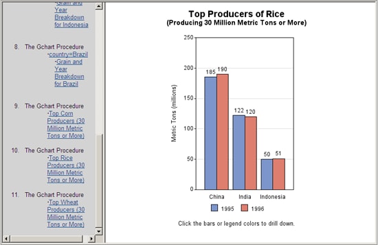
Finally the data is
charted by grain type. These graphs are linked to the bars in Browser View of Breakdown for China. If
you click the bar for
Rice, Browser View of Breakdown for Rice appears.Browser View of Breakdown for Rice
Overview: Part A
Part A of this program
creates the overview graph shown in Browser View of Overview Graph. In addition to setting the graphics
environment and creating the data set, Part A of the program does
the following:
-
Creates one grouped 2-D vertical bar chart (shown in Browser View of Overview Graph) with drill-down on the bars and legend values. The bars, represent total production for each year, for each country, are grouped and labeled by COUNTRY. Instead of displaying the year below each bar, the program suppresses the midpoint values with an AXIS statement and creates a legend that associates bar color and year. To create the legend, the chart variable YEAR is assigned to the SUBGROUP= option. Because the chart variable and the subgroup variable are the same, each bar contains only one "subgroup." As a result, the subgroup legend has an entry for each unique value of YEAR, thereby creating a legend for the midpoints. The values of COUNTRY label each group of bars.
Part A Program
filename odsout ".";
goptions reset=all xpixels=550 ypixels=500
   cback=white;
data grainldr;
   length country $ 3 type $ 5;
   input year country $ type $ amount;
   format megtons comma5.0;
   megtons=amount/1000;
datalines;
1995 BRZ Wheat 1516
1995 BRZ Rice 11236
1995 BRZ Corn 36276
1995 CHN Wheat 102207
1995 CHN Rice 185226
1995 CHN Corn 112331
1995 IND Wheat 63007
1995 IND Rice 122372
1995 IND Corn 9800
1995 INS Wheat .
1995 INS Rice 49860
1995 INS Corn 8223
1995 USA Wheat 59494
1995 USA Rice 7888
1995 USA Corn 187300
1996 BRZ Wheat 3302
1996 BRZ Rice 10035
1996 BRZ Corn 31975
1996 CHN Wheat 109000
1996 CHN Rice 190100
1996 CHN Corn 119350
1996 IND Wheat 62620
1996 IND Rice 120012
1996 IND Corn 8660
1996 INS Wheat .
1996 INS Rice 51165
1996 INS Corn 8925
1996 USA Wheat 62099
1996 USA Rice 7771
1996 USA Corn 236064
;
proc format;
   value $country
      "BRZ" = "Brazil"
      "CHN" = "China"
      "IND" = "India"
      "INS" = "Indonesia"
      "USA" = "United States";
data newgrain;
   set grainldr;
   length yeardrill typedrill countrydrill $ 100;

   /* Assign targets for the YEAR values. */
   yeardrill=
    "TITLE="||quote(trim(left(year)))||' '||
    "HREF="||quote('year'||trim(left(year))||'_body.html');

   /* Assign targets for the COUNTRY values. */
   countrydrill=
    "TITLE="||quote(trim(left(put(country,$country.))))||' '||
    "HREF="||quote('country_body.html#'||trim(left(country)));

   /* Assign targets for the TYPE values. */
   typedrill=
    "TITLE="||quote(trim(left(type)))||' '||
    "HREF="||quote(trim(left(type))||'_body.html');
legend1 label=none
   shape=bar(.15in,.15in)
   position=(bottom center);
ods html close;
goptions device=png;
ods html body="grain_body.html"
   frame="grain_frame.html"
   contents="grain_contents.html"
   gtitle gfootnote
   style=listing
   path=odsout;
axis1 label=none value=none;
axis2 label=(angle=90 "Metric Tons (millions)")
   minor=none
   order=(0 to 500 by 100)
   offset=(0,0);
axis3 label=none
   order=("China" "United States" "India" "Indonesia" "Brazil")
   split=" " offset=(4,4);
title1 ls=1.5 "Corn, Rice, and Wheat Production";
title2 "Leading Producers for 1995 and 1996";
footnote1 ls=1.3 "Click the bars or legend colors to drill down.";
proc gchart data=newgrain;
   format country $country.;
   vbar year / discrete type=sum sumvar=megtons
      group=country
      subgroup=year
      space=0
      maxis=axis1
      gaxis=axis3
      raxis=axis2
      autoref cref=graydd clipref
      legend=legend1
      html=countrydrill
      html_legend=yeardrill
      name="grainall"
      des="Overview of leading grain producers";
run;
quit;
Program Description
ODSOUT specifies a destination for the HTML and PNG files.The files are created in the example program. To
assign that location as the HTML destination for program output, ODSOUT
is specified later in the program in the ODS HTML statement's PATH=
option. ODSOUT must point to a Web location if procedure output is
to be viewed on the Web.
Set the graphics environment. The XPIXELS= and YPIXELS= options specify the size of each graph
as 550 pixels wide by 500 pixels high. The CBACK= option sets the
graph background to white.
Create the data set GRAINLDR. GRAINLDR contains data about grain production in five countries
for 1995 and 1996. The quantities in AMOUNT are in thousands of metric
tons. Variable MEGTONS stores the value of AMOUNT in millions of metric
tons.
data grainldr;
   length country $ 3 type $ 5;
   input year country $ type $ amount;
   format megtons comma5.0;
   megtons=amount/1000;
datalines;
1995 BRZ Wheat 1516
1995 BRZ Rice 11236
1995 BRZ Corn 36276
1995 CHN Wheat 102207
1995 CHN Rice 185226
1995 CHN Corn 112331
1995 IND Wheat 63007
1995 IND Rice 122372
1995 IND Corn 9800
1995 INS Wheat .
1995 INS Rice 49860
1995 INS Corn 8223
1995 USA Wheat 59494
1995 USA Rice 7888
1995 USA Corn 187300
1996 BRZ Wheat 3302
1996 BRZ Rice 10035
1996 BRZ Corn 31975
1996 CHN Wheat 109000
1996 CHN Rice 190100
1996 CHN Corn 119350
1996 IND Wheat 62620
1996 IND Rice 120012
1996 IND Corn 8660
1996 INS Wheat .
1996 INS Rice 51165
1996 INS Corn 8925
1996 USA Wheat 62099
1996 USA Rice 7771
1996 USA Corn 236064
;
proc format;
   value $country
      "BRZ" = "Brazil"
      "CHN" = "China"
      "IND" = "India"
      "INS" = "Indonesia"
      "USA" = "United States";
Add three HTML variables to GRAINLDR to create the NEWGRAIN
data set. Each HTML variable is assigned
the targets for a certain variable value. These targets are specified
by the HREF attribute within an AREA element in the HTML file. Each
HREF value specifies the HTML body file and, can also reference the
name of the anchor within the body file that identifies the target
graph. The HTML variable YEARDRILL contains the targets for the values
of the variable YEAR. The HTML variable COUNTRYDRILL contains the
targets for the values of the variable COUNTRY. The HTML variable
TYPEDRILL contains the names of the files that are the targets for
the values of the variable TYPE.
data newgrain;
   set grainldr;
   length yeardrill typedrill countrydrill $ 100;

   /* Assign targets for the YEAR values. */
   yeardrill=
    "TITLE="||quote(trim(left(year)))||' '||
    "HREF="||quote('year'||trim(left(year))||'_body.html');

   /* Assign targets for the COUNTRY values. */
   countrydrill=
    "TITLE="||quote(trim(left(put(country,$country.))))||' '||
    "HREF="||quote('country_body.html#'||trim(left(country)));

   /* Assign targets for the TYPE values. */
   typedrill=
    "TITLE="||quote(trim(left(type)))||' '||
    "HREF="||quote(trim(left(type))||'_body.html');
Define legend characteristics for all legends. SHAPE= specifies the shape and size of the legend
entries. POSITION= specfieis the position of the legend.
Open the ODS HTML destination for the ODS graphics output. BODY= names the file for storing the HTML output.
FRAME= names the HTML file that integrates the contents and body files.
CONTENTS= names the HTML file that contains the table of contents
to the HTML procedure output. The contents file links to each of the
body files written to the HTML destination. GTITLE includes the graph
title in the SAS/GRAPH output instead of the HTML output. PATH= specifies
the ODSOUT fileref as the HTML destination for all the HTML and PNG
files.
ods html body="grain_body.html"
   frame="grain_frame.html"
   contents="grain_contents.html"
   gtitle gfootnote
   style=listing
   path=odsout;
Suppress the label and values for the midpoint axis.The midpoint values 1995 and 1996 do not appear below
each bar.
Modify the response axis. The LABEL= option specifies a new axis label and rotates it 90 degrees.
The MINOR=NONE option suppresses the minor tick marks. The ORDER=
option sets the response axis range to 0 to 500 in increments of 100.
The OFFSET= option sets the offsets to zero.
Suppress the label and order the values for the group
axis. Because the values of COUNTRY
are formatted, ORDER= must specify their formatted value.
axis3 label=none
   order=("China" "United States" "India" "Indonesia" "Brazil")
   split=" " offset=(4,4);
title1 ls=1.5 "Corn, Rice, and Wheat Production";
title2 "Leading Producers for 1995 and 1996";
footnote1 ls=1.3 "Click the bars or legend colors to drill down.";
Generate the vertical bar chart that summarizes all grain
production for all countries for both years.DISCRETE creates a separate bar for each unique value
of YEAR. GROUP= groups the bars by country. To create a legend for
midpoint values, SUBGROUP= is assigned the chart variable YEAR. SPACE=
controls the space between the bars. HTML= specifies COUNTRYDRILL
as the variable that contains the targets for the bars. Because the
COUNTRYDRILL variable contains the TITLE= and HREF= options, the URL=
option cannot be used in this case. HTML_LEGEND= specifies YEARDRILL
as the variable that contains the targets for the legend values. Specifying
HTML variables causes SAS/GRAPH to add an image map to the HTML body
file. NAME= specifies the name of the catalog entry. Because the PATH=
destination is a file storage location and not a specific filename,
the catalog entry name GRAINALL is automatically assigned to the PNG
file. DES= specifies the description that is stored in the graphics
catalog and used in the Table of Contents.
proc gchart data=newgrain;
   format country $country.;
   vbar year / discrete type=sum sumvar=megtons
      group=country
      subgroup=year
      space=0
      maxis=axis1
      gaxis=axis3
      raxis=axis2
      autoref cref=graydd clipref
      legend=legend1
      html=countrydrill
      html_legend=yeardrill
      name="grainall"
      des="Overview of leading grain producers";
run;
quit;
Overview: Part B
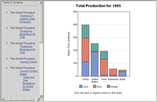
Part B of this program
creates the two charts that show the grain production breakdown by
year for 1995 and 1996. The chart for 1995 is shown in Browser View of Year Breakdown for 1995. Each bar in
these graphs represents a country and is subgrouped by grain type.
As before, both the bars and the legend values are links to other
graphs. The bars link to targets stored in COUNTRYDRILL, and the legend
values link to targets in TYPEDRILL. These two graphs not
only contain links, they are the link targets for the legend values in Browser View of Overview Graph, Browser View of Breakdown for Rice, and Browser View of Breakdown for China. Before each graph is generated, the ODS HTML statement
opens a new body file in which to store the output. Because each of
these graphs is stored in a separate file, the HREF attributes that
are stored in the variable YEARDRILL point only to the file. The name
of the file is specified by the BODY= option in the ODS HTML statement.
Here is an example of the HREF attribute that points to the graph
of 1995 and is stored in the variable YEARDRILL:
HREF=year1995_body.htmlYEARDRILL is assigned to the HTML_LEGEND= option in Part A.
Part B Program
axis4 label=none
   order=("China" "United States" "India" "Indonesia" "Brazil")
   split=" " offset=(8,8);
%macro do_year(year);
ods html body="year&year._body.html"
  gtitle gfootnote
  path=odsout style=listing;
title1 ls=1.5 "Total Production for &year";
proc gchart data=newgrain (where=(year=&year));
   format country $country.;
   vbar country / type=sum sumvar=megtons
      subgroup=type
      legend=legend1
      raxis=axis2
      maxis=axis4
      width=8
      autoref cref=graydd clipref
      html=countrydrill
      html_legend=typedrill
      name="year_&year"
      des="Production Breakdown for &year";
run;
quit;
%mend do_year;
%do_year(1995);
%do_year(1996);
Program Description
Suppress the label and order the values for the midpoint
axis.The ORDER= option specifies the
new order for the midpoints. The SPLIT=“ ” option allows
the labels to wrap on a blank space, if necessary.
axis4 label=none
   order=("China" "United States" "India" "Indonesia" "Brazil")
   split=" " offset=(8,8);
Open a new body file for the graph of production for
the year specified. Assigning a new
body file closes GRAIN_BODY.HTML. The body filename includes the year
that is passed into the macro so that it can be identified easily.
The contents and frame files, which remain open, and provide links
to all body files.
Subset the data for the year that is passed into the macro
and generate the vertical bar chart for that year. The AUTOREF option draws a reference line on the
backplane for every major tick mark value. The SUBGROUP= option creates
a separate bar segment for each department. The HTML= option names
the variable that contains the targets for the bars. The HTML_LEGEND=
option names the variable that contains the targets for the legend
values. The PNG files use the catalog entry name specified by the
NAME= option. The name and description include the year that is passed
into the macro.
proc gchart data=newgrain (where=(year=&year));
   format country $country.;
   vbar country / type=sum sumvar=megtons
      subgroup=type
      legend=legend1
      raxis=axis2
      maxis=axis4
      width=8
      autoref cref=graydd clipref
      html=countrydrill
      html_legend=typedrill
      name="year_&year"
      des="Production Breakdown for &year";
run;
quit;Overview: Part C
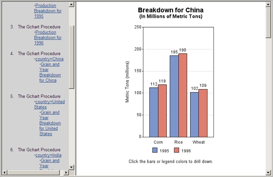
Part C of this program
produces the five graphs that show the breakdowns by country. The
chart for China is shown in Browser View of Breakdown for China. Macro %DO_COUNTRY is defined and used to generate the
graphs for each country, and all of the graphs are stored in a one
file. When the file is displayed in the browser, all the graphs appear
in one frame that can be scrolled. Because the graphs are stored in
one file, the links to them must explicitly point to the location
of each graph in the file, not just to the file. This location is
defined by an anchor. ODS HTML assigns anchor names by default, but
you can specify anchor names with the ANCHOR= option. This program
assigns a name {COUNTRY} to the ANCHOR= variable value for each country.
The graphs created by this part are referenced by the COUNTRYDRILL
variable. The NAME= option specifies “country_country” as the name for the graphics
output for each country. The DES= option specifies a generic description
for the HTML Table of Contents.
Part C Program
axis5 label=none split=" " offset=(4,4);
axis6 label=(angle=90 "Metric Tons (millions)")
   minor=none
   order=(0 to 250 by 50)
   offset=(0,0);
ods html body="country_body.html"
  gtitle gfootnote
  path=odsout style=listing;
options nobyline;
%macro do_country(country);
ods html anchor="&country";
title1 ls=1.5 "Breakdown for #byval(country)";
title2 "(In Millions of Metric Tons)";
proc gchart data=newgrain (where=(country="&country"));
   format country $country.;
   by country;  /* Enables the use of #byval() in title and description */
   vbar year / discrete type=sum sumvar=megtons
      group=type
      subgroup=year
      legend=legend1
      outside=sum
      space=0
      maxis=axis1
      raxis=axis6
      gaxis=axis5
      autoref cref=graydd clipref
      html=typedrill
      html_legend=yeardrill
      name="country_&country"
      des="Grain and Year Breakdown for #byval(country)";
run;
%mend do_country;
%do_country(CHN);
%do_country(USA);
%do_country(IND);
%do_country(INS);
%do_country(BRZ);

quit;
Program Description
Generate the vertical bar chart of production for each
country.BY-group processing on variable
COUNTRY is used here so that #BYVAL(COUNTRY) can be used in the TITLE1
statement and the DES= procedure option. Since the WHERE clause in
the DATA= procedure option filters the data to include only one country,
only one output file is generated per macro call in this case. The
GROUP= option groups the bars by country. The OUTSIDE= option displays
the SUM statistic above the bars. The HTML= option specifies TYPEDRILL
as the variable that contains the targets for the bars. Because the
TYPEDRILL variable contains the TITLE= and HREF= options, the URL=
option cannot be used in this case. The RAXIS= option assigns the
AXIS4 statement . The GAXIS= option assigns the AXIS5 statement. The
MAXIS= option assigns the AXIS1 statement to the midpoint axis. The
NAME= option specifies the name of the catalog entry. The graphics
catalog entry name increments so the PNG files are named sequentially
from COUNTRY to COUNTRY4. The DES= option specifies a general description
that appears in the table of contents for all five graphs.
proc gchart data=newgrain (where=(country="&country"));
   format country $country.;
   by country;  /* Enables the use of #byval() in title and description */
   vbar year / discrete type=sum sumvar=megtons
      group=type
      subgroup=year
      legend=legend1
      outside=sum
      space=0
      maxis=axis1
      raxis=axis6
      gaxis=axis5
      autoref cref=graydd clipref
      html=typedrill
      html_legend=yeardrill
      name="country_&country"
      des="Grain and Year Breakdown for #byval(country)";
run;
Overview: Part D
Part C of this program
creates the charts that show the leading producers for each type of
grain. The chart for rice is shown in Browser View of Breakdown for Rice. This part of the program defines
and uses macro %DO_TYPE to generate graphs that show the leading producers
for each type of grain. A leading producer is defined as any producer
that produces 30 metric megatons or more of grain. The program subsets
the data and suppresses midpoints with no observations. Instead of
storing all of the output in one body file, it stores each graph in
a separate file using the ODS HTML option NEWFILE=TABLE. Because
each graph is stored in a separate file, the links to these graphs
reference filename only and do not require an anchor name. The graphs
created by this part are referenced by the TYPEDRILL variable.
Part D Program
%macro do_type(type);
ods html body="&type._body.html"
  newfile=table
  gtitle gfootnote
  path=odsout style=listing;
%let minamount=30;
title1 ls=1.5 "Top Producers of &type";
title2 "(Producing &minamount Million Metric Tons or More)";
/* Produce the series of bar charts: country and type. */
proc gchart data=newgrain (where=(megtons ge &minamount and type="&type"));
   format country $country.;
   vbar year / discrete type=sum sumvar=megtons
      group=country
      subgroup=year
      legend=legend1
      outside=sum
      space=0
      maxis=axis1
      raxis=axis6
      gaxis=axis5
      autoref cref=graydd clipref
      html=countrydrill
      html_legend=yeardrill
      name="type_&type"
      des="Top &type Producers (&minamount Million Metric Tons or More)";
run;
quit;
%mend do_type;
%do_type(Corn);
%do_type(Rice);
%do_type(Wheat);
title;
footnote;
ods html close;
ods html;
Program Description
Open a new body file. Assigning
a new body file closes COUNTRY_BODY.HTML. NEWFILE=TABLE opens a new
body file for each piece of output generated by the procedure.
Define the lower threshold for the top producers.MINAMOUNT is the minimum amount of grain that a producer
must product in order to be considered a top producer. The value is
expressed in metric megatons.
title1 ls=1.5 "Top Producers of &type";
title2 "(Producing &minamount Million Metric Tons or More)";
/* Produce the series of bar charts: country and type. */
proc gchart data=newgrain (where=(megtons ge &minamount and type="&type"));
   format country $country.;
   vbar year / discrete type=sum sumvar=megtons
      group=country
      subgroup=year
      legend=legend1
      outside=sum
      space=0
      maxis=axis1
      raxis=axis6
      gaxis=axis5
      autoref cref=graydd clipref
      html=countrydrill
      html_legend=yeardrill
      name="type_&type"
      des="Top &type Producers (&minamount Million Metric Tons or More)";
run;
quit;
Example 3: Creating a Drill-Down Java Presentation for the Web
| Features: |
VBAR3D Statement
|
| Other features: |
|
The Graph applet is
a Java applet that provides drill-down functionality by default. You
do not need to add linking variables to your chart data to get drill-down
links when using the Graph applet. To use the Graph applet to generate
your graph, use the DEVICE=JAVA graphics option. When the Web page
is displayed, the drill-down functionality is enabled by default.
The Graph applet retains the type and style of the initial graph for
all the graphs in the presentation. This example creates a drill-down
sequence of three-dimensional, vertical bar charts that use the ODS
style LISTING.
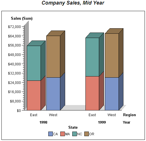
The initial graph displayed
by this example is shown in the following figure. In this graph, REGION
is the independent variable, and SALES is the dependent variable.
YEAR is the group variable, and STATE is the subgroup variable.
Graph Applet: Level 1
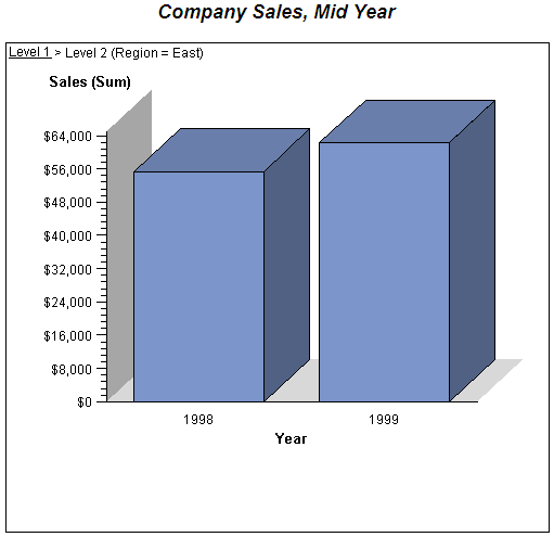
Clicking the bar segment
labeled East generates the graph shown in Graph Applet: Level 2 . The Level
2 drill-down graph retains the dependent variable SALES. The group
variable YEAR is promoted to the independent variable role. The drill-down
action creates one bar segment for each unique value of YEAR. SALES
is the dependent variable, and YEAR is the independent variable.
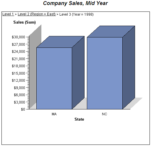
Clicking the bar segment
labeled 1998 generates the graph shown in Graph Applet: Level 3 . The Level
3 drill-down graph retains the dependent variable SALES. The subgroup
variable STATE is promoted to the independent variable role. STATE
is the last variable that can appear as an independent variable. The
drill-down action creates one bar segment for each unique value of
STATE. SALES is the dependent variable, and STATE is the independent
variable.
Program
/* Create the temporary data set named sales. */ data sales; length Region $ 4 State $ 2; format Sales dollar8.; input Region State Sales Year Qtr; datalines; West CA 13636 1999 1 West OR 18988 1999 1 West CA 14523 1999 2 West OR 18988 1999 2 East MA 18038 1999 1 East NC 13611 1999 1 East MA 11084 1999 2 East NC 19660 1999 2 West CA 12536 1998 1 West OR 17888 1998 1 West CA 15623 1998 2 West OR 17963 1998 2 East NC 17638 1998 1 East MA 12811 1998 1 East NC 12184 1998 2 East MA 12760 1998 2 ; /* Specify the JAVA device for generating the chart. */ goptions reset=all border device=java; /* Close the current ODS HTML destination. */ ods html close; /* Open the HTML destination. Specify vbarweb.htm as */ /* the output filename and GEARS as the style. */ ods html file="vbarweb.htm" style=listing; /* Generate the bar chart. Group by YEAR and subgroup */ /* by STATE. */ title "Company Sales, Mid Year"; proc gchart data=sales; vbar3d region / sumvar=sales group=year subgroup=state; run; quit; /* ODS html to close the output file, and then reopen ODS HTML. */ ods html close; ods html;
Example 4: Enhancing an SVG Drill-Down Presentation Using HTML Attributes
| Features: |
VBAR statement
GREPLAY DELETE statement |
| Other features: |
BY-Group processing
OPTIONS statement NOBYLINE option |
This example uses the
SVG graphics device with the ONMOUSEOVER= HTML attribute in the HTML=
string to add special effects to a drill-down graph. The drill-down
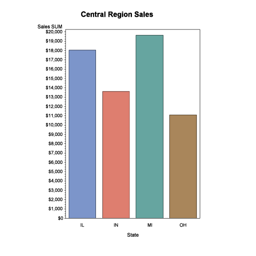
graph is a simple bar chart of regional sales data. Each bar in the
main chart is linked to a drill-down graph that displays detailed
sales data for that region. The special effects are activated when
the mouse pointer is positioned on a bar. The drill-down link for
each bar contains the ONMOUSEOVER= HTML attribute. The ONMOUSEOVER=
HTML attribute value includes the showImage and changeOpacity functions.
The showImage function displays a pop–up preview image of a
bar’s drill-down chart in the upper right corner of the graph
when the mouse pointer is positioned on that bar. The changeOpacity
function changes the fill opacity of a bar to 50% when the mouse pointer
is positioned on that bar. When a bar is clicked, an enlarged version
of the drill-down graph for that bar opens in the browser window.
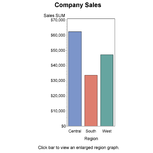
The main graph is stored
in file SALESREPORT.HTML. Here is the graph as it is initially displayed
when this file is opened.
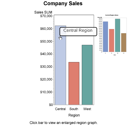
When the mouse pointer
is positioned on the Central bar, for example, the fill opacity of
the bar changes to 50%, and a pop–up image of the Central Region
Sales drill-down chart is displayed in the top right corner of the
graphics output area as shown in the following figure.
Program
filename gout ".";
data regsales(drop=drillurl imgurl);
length Region State $8 drillurl imgurl $50 htmlstr $256;
format Sales dollar8.;
input Region State Sales drillurl imgurl;
/* Create and add the HTML variable for each observation. */
htmlstr="href="||quote(trim(drillurl))||
" title="||quote(trim(Region)||" Region") ||
" ONMOUSEOVER=ShowImage("||quote(trim(imgurl))||
",400,25,200,200); changeOpacity(.5)";
datalines;
Central IL 18038 ./regsales.html#rpt ./sales.svg
Central IN 13611 ./regsales.html#rpt ./sales.svg
Central OH 11084 ./regsales.html#rpt ./sales.svg
Central MI 19660 ./regsales.html#rpt ./sales.svg
South FL 14541 ./regsales.html#rpt1 ./sales1.svg
South GA 19022 ./regsales.html#rpt1 ./sales1.svg
West CA 13636 ./regsales.html#rpt2 ./sales2.svg
West OR 18988 ./regsales.html#rpt2 ./sales2.svg
West WA 14523 ./regsales.html#rpt2 ./sales2.svg
;
goptions reset=all border device=svg xpixels=600 ypixels=450;
ods html close;
ods html body="salesreport.html" path=gout style=listing
parameters=("drilldownmode"="html");
title1 "Company Sales"; footnote1 j=c "Click bar to view an enlarged region graph."; proc gchart data=regsales; vbar region / sumvar=sales width=8 patternid=midpoint html=htmlstr; /* Set the HTML variable to htmlstr. */ run; quit;
ods html close;
proc greplay nofs igout=work.gseg; delete _all_; run; quit;
goptions reset=all border device=svgt;
options nobyline;
ods html body="regsales.html" path=gout anchor="rpt" style=listing;
title "#byval(region) Region Sales"; proc gchart data=regsales; vbar state / sumvar=sales width=10 name="sales" patternid=midpoint; by region; run; quit;
ods html close;
ods html;
Program Description
Set the file output path.By default, ODS sends its output to the SAS Work directory. You can
create a fileref to specify a different location for your ODS output,
which is done later in this program.
Create the sales data set.The data set includes the region name, state codes, and the regional
sales figures. It also includes the drill-down URL for each the drill-down
graphs (DRILLURL) and the path to the pop-up image for each drill-down
graph (IMGURL). Notice that the base anchor RPT is used in the drill-down
URLs. This base anchor is specified later in this program. The HTMLSTR
variable is added to the data for each observation to store the HTML
drill-down string. It is formed from the DRILLURL and IMGURL variables,
and includes the TITLE= and ONMOUSEOVER= HTML attributes. The ONMOUSEOVER=
HTML attribute value contains the ShowImage and changeOpacity functions
to achieve the desired effects. After the HTMLSTR variable is formed,
the DRILLURL and IMGURL variables are no longer needed and are dropped
from the data set.
data regsales(drop=drillurl imgurl);
   length Region State $8 drillurl imgurl $50 htmlstr $256;
   format Sales dollar8.;
   input Region State Sales drillurl imgurl;

   /* Create and add the HTML variable for each observation. */
   htmlstr="href="||quote(trim(drillurl))||
      " title="||quote(trim(Region)||" Region") ||
      " ONMOUSEOVER=ShowImage("||quote(trim(imgurl))||
      ",400,25,200,200); changeOpacity(.5)";

datalines;
Central IL 18038 ./regsales.html#rpt  ./sales.svg
Central IN 13611 ./regsales.html#rpt  ./sales.svg
Central OH 11084 ./regsales.html#rpt  ./sales.svg
Central MI 19660 ./regsales.html#rpt  ./sales.svg
South   FL 14541 ./regsales.html#rpt1 ./sales1.svg
South   GA 19022 ./regsales.html#rpt1 ./sales1.svg
West    CA 13636 ./regsales.html#rpt2 ./sales2.svg
West    OR 18988 ./regsales.html#rpt2 ./sales2.svg
West    WA 14523 ./regsales.html#rpt2 ./sales2.svg
;Set the graphics options for the top-level graph.The SVG graphics device is used for the top-level
graph.
Specify the ODS HTML settings for the top-level graph. The top-level graph output is sent to file SALESREPORT.HTML
in the directory that was defined earlier by fileref GOUT (the current
directory in this example). The LISTING style is used for this graph.
The drill-down mode is set to HTML.
title1 "Company Sales";
footnote1 j=c "Click bar to view an enlarged region graph.";
proc gchart data=regsales;
   vbar region / sumvar=sales width=8
   patternid=midpoint
   html=htmlstr; /* Set the HTML variable to htmlstr. */
run;
quit;
Clear the GRSEG catalog. Because the image files must be SALES.SVG, SALES1.SVG, and SALES2.SVG,
as defined in variable IMGURL in the data set, the existing SALES
entries must be cleared from the GRSEG catalog. Otherwise, different
filenames might be used. In that case, the pop-up images will not
display.
Specify the graphics options for the drill-down graphs. Because the drill-down graph images are overlaid
onto the main graph, the SVGT device is used for the drill-down graphs
so that the background of the main graph shows through the pop-up
graph images.
Suppress the BY line. BY-group
processing is used to generate the drill-down graphs. To suppress
the BY line in the drill-down graphs, set the NOBYLINE system option.
Specify the ODS HTML settings for the drill-down graphs. The drill-down graphs are stored in file REGSALES.HTML
in the directory that is defined by fileref GOUT. The ANCHOR=RPT sets
the base anchor to RPT, which is specified in the DRILLURL variable
in the data set.