DSGI Graphics Summary
The following sections summarize the functions and
routines that you can use to create graphics output with DSGI.
DSGI Functions
DATA Step Graphics Interface Functions summarizes the types of operations available and the functions
used to invoke them. Refer to The DSGI Function and Routine Dictionaries for details about each function.
DSGI Routines
DSGI routines return
the values set by some of the DSGI functions. DATA Step Graphics Interface Routines summarizes the types of values that the GASK routines can
check. Refer to The DSGI Function and Routine Dictionaries for details about each routine.
Creating Simple Graphics with DSGI
Basic Steps to Create DSGI Output
Basic Steps Used in Creating DSGI Graphics Output outlines the basic steps and shows the functions used to
initiate steps 1, 2, 4, and 5. Step 3 can consist of many types of
functions. The GDRAW(“LINE”, . . . ) function is used
as an example.
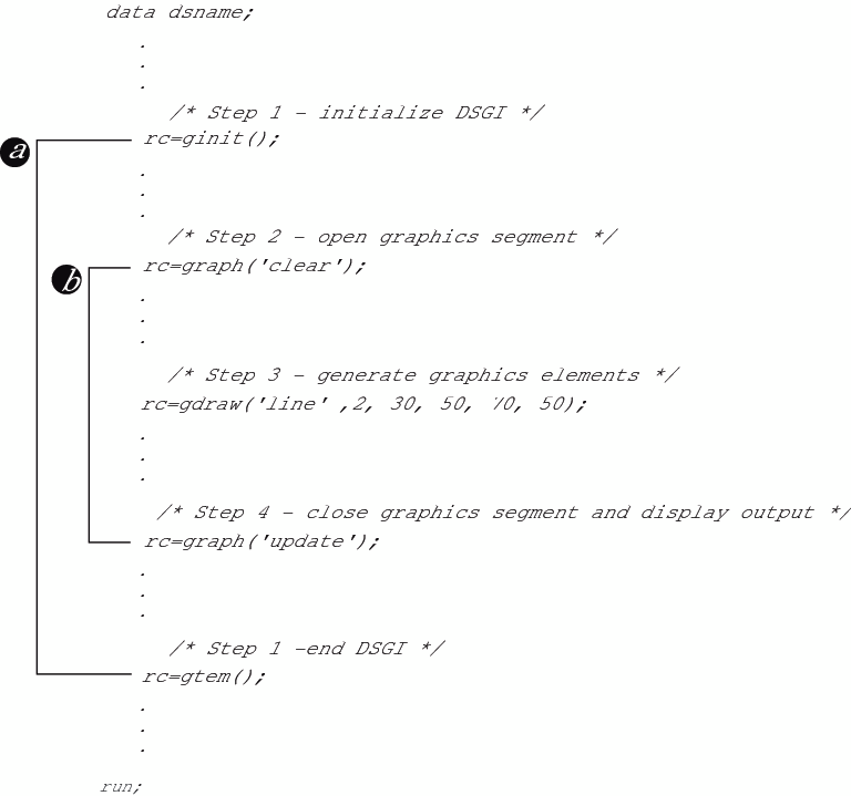
Notice that there are
two pairs of functions that work together within a DSGI DATA step
(shown by a and b in Basic Steps Used in Creating DSGI Graphics Output.) The first pair, GINIT() and GTERM(), begin and end DSGI.
Within the first pair, the second pair, GRAPH(“CLEAR”,
. . . ) and GRAPH(“UPDATE”, . . . ) begin and end a
graphics segment. You can repeat these pairs within a single DATA
step to produce multiple graphics output. However, the relative positions
of these functions must be maintained within a DATA step. See Generating Multiple Graphics Output in One DATA Step for more information about producing multiple graphics
outputs from one DATA step.
The order of these steps
is controlled by DSGI operating states. Before any DSGI function or
routine can be submitted, the operating state in which that function
or routine can be submitted must be active. See How Operating States Control the Order of DSGI Statements.
Setting Attributes for Graphics Elements
The appearance of the
graphics elements is determined by the settings of the attributes.
Attributes control such aspects as height of text; text font; and
color, size, and width of the graphics element. In addition, the HTML
attribute determines whether the element provides a link to another
graphic or web page. Attributes are set and reset with GSET functions.
GASK routines return the current setting of the attribute specified.
Each graphics primitive
is associated with a particular set of attributes. Its appearance
or linking capability can be altered only by that set of attributes. Graphics Output Primitive Functions and Associated Attributes lists the operators used with GDRAW functions to generate
graphics elements and the attributes that control them.
Attribute functions
must precede the graphics primitive they control. Once an attribute
is set, it controls any associated graphics primitives that follow.
If you want to change the setting, you can issue another GSET(attribute, . . . ) function with the new setting.
If you do not set an
attribute before you submit a graphics primitive, DSGI uses the default
value for the attribute. Refer to The DSGI Function and Routine Dictionaries for the default values used for each attribute.
Functions That Change the Operating State
The functions described
earlier in steps 1, 2, 4, and 5 actually control the changes to the
operating state. For example, the GINIT() function must be submitted
when the operating state is GKCL, the initial state of DSGI. GINIT()
then changes the operating state to WSAC. The GRAPH(“CLEAR”,
. . . ) function must be submitted when the operating state is WSAC
and before any graphics primitives are submitted. The reason it precedes
graphics primitives is that it changes the operating state to SGOP,
the operating state in which you can submit graphics primitives.
The following list shows the change in the operating state due to
specific functions:
Because these functions
change the operating state, you must order all other functions and
routines so that the change in operating state is appropriate for
the functions and routines that follow. The following program statements
show how the operating state changes from step to step in a typical
DSGI program. They also summarize the functions and routines that
can be submitted under each operating state. The functions that change
the operating state are included as actual statements. Refer to The DSGI Function and Routine Dictionaries for the operating states from which functions and routines
can be submitted.
data dsname;
/* GKCL - initial state of DSGI; can execute: */
/* 1. GSET functions that set attributes */
/* that affect the entire graphics output */
/* 2. some catalog management functions */
/* (some GRAPH functions) */
/* Step 1 - initialize DSGI */
rc=ginit();
/* WSAC - workstation is active; can execute: */
/* 1. most GASK routines */
/* 2. some catalog management functions */
/* (some GRAPH functions) */
/* 3. GSET functions that set attributes */
/* and bundles, viewports, windows, */
/* transformations, and message logging */
/* Step 2 - open a graphics segment */
rc=graph("clear", "text");
/* SGOP - segment open; can execute: */
/* 1. any GASK routine */
/* 2. any GDRAW function */
/* 3. some catalog management functions */
/* (some GRAPH functions) */
/* 4. GSET functions that set attributes */
/* and bundles, viewports, windows, */
/* transformations, and message logging */
/* Step 3 - execute graphics primitives */
rc = gdraw("line", 2, 30,50,50,50);
/* Step 4 - close the graphics segment */
rc=graph("update");
/* WSAC - workstation is active; can execute: */
/* 1. most GASK routines */
/* 2. some catalog management functions */
/* (some GRAPH functions) */
/* 3. GSET functions that set attributes */
/* and bundles, viewports, windows, */
/* transformations, and message logging */
/* Step 5 - end DSGI */
rc=gterm();
/* GKCL - initial state of DSGI */
run;Order of Functions and Routines
Functions and routines
within each operating state can technically be submitted in any order.
However, once an attribute is set, it remains in effect until the
end of the DATA step or until you change its value. If you are producing
multiple graphics output within the same DATA step, the attributes
for one output affect the ones that follow. Attributes are not reset
until after the GTERM() function is submitted.
Notice that you can
set attributes for the graphics primitives in several places. As
long as the functions that set the attributes are executed before
the graphics primitives, they affect the graphics output. If you
execute them after a graphics primitive, the primitive is not affected.
See Setting Attributes for Graphics Elements.
The following program
statements illustrate a more complex DSGI program that produces Simple Graphics Output Generated with DSGI when submitted. Notice that all attributes for a graphics
primitive are executed before the graphics primitive. In addition,
the GINIT() and GTERM() pairing and the GRAPH(“CLEAR”)
and GRAPH(“UPDATE”) pairing are maintained within the
DATA step. Refer to The DSGI Function and Routine Dictionaries for the operating states in which each function and routine
can be submitted.
/* set the graphics environment */
goptions reset=global gunit=pct border
hsize=7 in vsize=5 in
targetdevice=pscolor;
/* execute a DATA step with DSGI */
data dsname;
/* initialize
SAS/GRAPH software */
/* to accept DSGI statements */
rc=ginit();
rc=graph("clear");
/* assign colors to color index */
rc=gset("colrep", 1, "blue");
rc=gset("colrep", 2, "red");
/* define and display titles */
rc=gset("texcolor", 1);
rc=gset("texfont", "swissb");
rc=gset("texheight", 6);
rc=gdraw("text", 45, 93, "Simple Graphics Output");
/* change the height and */
/* display second title */
rc=gset("texheight", 4);
rc=gdraw("text", 58, 85, "Created with DSGI");
/* define and display footnotes */
/* using same text font and */
/* color as defined for titles */
rc=gset("texheight", 3);
rc=gdraw("text", 125, 1, "GDSORDER ");
/* define and draw bar */
rc=gset("lincolor", 2);
rc=gset("linwidth", 5);
rc=gdraw("line", 2, 72, 72, 30, 70);
rc=gdraw("line", 2, 52, 92, 50, 50);
/* display graph and end DSGI */
rc=graph("update");
rc=gterm();
run;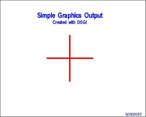
Bundling Attributes
Overview of Bundling Attributes
Attributes That Can Be Bundled for Each Graphics Primitive
Each graphics primitive
has a group of attributes associated with it that can be bundled.
Only the attributes in that group can be assigned to the bundle.
Attributes That Can Be Bundled for Each Graphics Primitive shows the attributes that can be bundled for each graphics
primitive.
Note: You do not have to use attribute
bundles for all graphics primitives if you use a bundle for one.
You can define bundles for some graphics primitives and set the attributes
individually for others.
However, if the other
graphics primitives are associated with the same attributes that you
have bundled and you do not want to use the same values, you can use
other bundles to set the attributes, or you can set the attributes
back to “INDIVIDUAL”.
Assigning Attributes to a Bundle
To assign values of
attributes to a bundle, you must do the following:
-
assign the values to a numeric bundle index with the GSET(“xxx REP”, . . . ) function. Each set of attributes that can be bundled uses a separate GSET(“xxx REP”, . . . ) function, where xxx is the appropriate prefix for the set of attributes to be bundled. Valid values for xxx are FIL, LIN, MAR, and TEX.
The following example
assigns the text attributes, color, and font, to the bundle indexed
by the number 1. As shown in the GSET(“TEXREP”, . .
. ) function, the color for the bundle is green, the second color
in the COLOR= graphics option. The font for the bundle is the “ZAPF”
font. (See Using Colors in SAS/GRAPH Programs for an explanation of how colors are used in DSGI.)
goptions colors=(red green blue);
data dsname;
.
. /* other DATA step statements */
.
/* associate the bundle with the index 1 */
rc=gset("texrep", 1, 2, "zapf");
.
. /* more statements */
.
/* assign the text attributes to a bundle */
rc=gset("asf", "texcolor", "bundled");
rc=gset("asf", "texfont", "bundled");
/* draw the text */
rc=gdraw("text", 50, 50, "Today is the day.");Selecting a Bundle
Once you have issued
the GSET(“ASF”, . . . ) and GSET(“xxx REP”, . . . ) functions, you can issue
the GSET(“xxx INDEX”,
. . . ) function to select the bundle. The following statement selects
the bundle defined in the previous example:
/* invoke the bundle of text attributes */
rc=gset("texindex", 1);Defining Multiple Bundles for a Graphics Primitive
You can set up more
than one bundle for graphics primitives by issuing another GSET(“xxx REP”, . . . ) function with a different
index number. If you wanted to add a second attribute bundle for
text to the previous example, you could issue the following statement:
/* define another attribute bundle for text */
rc=gset("texrep", 2, 3, "swiss");When you activate the
second bundle, the graphics primitives for the text that follows uses
the third color, blue, and the SWISS font.
How DSGI Selects the Value of an Attribute to Use
Attributes that are
bundled override any of the same attributes that are individually
set. For example, you assign the line color green, the type 1, and
the width 5 to a line bundle with the following statements:
goptions colors=(red green blue);
rc=gset("asf", "lincolor", "bundled");
rc=gset("asf", "linwidth", "bundled");
rc=gset("asf", "lintype", "bundled");
rc=gset("linrep", 3, 2, 5, 1);In subsequent statements,
you activate the bundle, select other attributes for the line, and
then draw a line:
/* activate the bundle */
rc=gset("linindex", 3);
/* select other attributes for the line */
rc=gset("lincolor", 3);
rc=gset("linwidth", 10);
rc=gset("lintype", 4);
/* draw a line from point (30,50) to (70,50) */
rc=gdraw("line", 2, 30, 70, 50, 50);The color, type, and
width associated with the line bundle are used rather than the attributes
set just before the GDRAW(“LINE”, . . . ) function was
executed. The line that is drawn is green (the second color from the
color list of the COLORS= graphics option), five units wide, and solid
(line type 1).
Disassociating an Attribute from a Bundle
To disassociate an attribute
from a bundle, use the GSET(“ASF”, . . . ) function
to reset the ASF of the attribute to “INDIVIDUAL”.
The following program statements demonstrate how to disassociate the
attributes from the text bundle:
/* disassociate an attribute from a bundle */
rc=gset("asf", "texcolor", "individual");
rc=gset("asf", "texfont", "individual");Using Viewports and Windows
Overview of Using Viewports and Windows
In DSGI, you can
define viewports and windows. Viewports enable you to subdivide the
graphics output area and insert existing graphs or draw graphics elements
in smaller sections of the graphics output area. Windows define the
coordinate system within a viewport and enable you to scale the graph
or graphics elements drawn within the viewport.
The default viewport
is defined as (0,0) to (1,1) with 1 being 100% of the graphics output
area. If you do not define a viewport, graphics elements or graphs
are drawn using the default.
The default window is
defined so that a rectangle drawn from window coordinates (0,0) to
(100,100) is square and fills the display in one dimension. The actual
dimensions of the default window are device dependent. Use the GASK(“WINDOW”, . . . ) routine to find the exact dimensions of your default window. You
can define a window without defining a viewport. The coordinate system
of the window is used with the default viewport.
If you define a viewport,
you can position it anywhere in the graphics output area. You can
define multiple viewports within the graphics output area so that
more than one existing graph, part of a graph, or more than one graphics
element can be inserted into the graphics output.
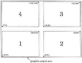
Transformations activate
both a viewport and the associated window. DSGI maintains 21 (0 through
20) transformations. By default, transformation 0 is active. Transformation
0 always uses the entire graphics output area for the viewport, and
maps the window coordinates to fill the viewport. The definition of
the viewport and window of transformation 0, cannot be changed.
By default, the viewports
and windows of all the other transformations (1 through 20) are set
to the defaults for viewports and windows. If you want to define a
different viewport or window, you must select a transformation number
between 1 and 20.
These steps can be submitted
in any order. However, if you use a transformation that you have not
defined, the default viewport and window are used. Once you activate
a transformation, the graphics elements drawn by the subsequent DSGI
functions are drawn in the viewport and window associated with that
transformation.
Defining Viewports
You can define a viewport
with the GSET(“VIEWPORT”, n, . . . ) function, where n is the transformation number of the viewport that you are defining.
You can also use this function to define multiple viewports, each
containing a portion of the graphics output area. You can then place
a separate graph, part of a graph, or graphics elements within each
viewport.
The following program
statements divide the graphics output area into four subareas:
/* define the first viewport, indexed by 1 */
rc=gset("viewport", 1, .05, .05, .45, .45);
/* define the second viewport, indexed by 2 */
rc=gset("viewport", 2, .55, .05, .95, .45);
/* define the third viewport, indexed by 3 */
rc=gset("viewport", 3, .55, .55, .95, .95);
/* define the fourth viewport, indexed by 4 */
rc=gset("viewport", 4, .05, .55, .45, .95);Clipping around Viewports
When you use viewports,
you also might need to use the clipping feature. Even though you have
defined the dimensions of your viewport, it is possible for graphics
elements to display past its boundaries. If the graphics elements
are too large to fit into the dimensions that you have defined, portions
of the graphics elements actually display outside of the viewport.
To ensure that only the portions of the graphics elements that fit
within the dimensions of the viewport display, turn the clipping feature
on by using the GSET(“CLIP”, . . . ) function. For details,
see CLIP.
Defining Windows
You can define a window
by using the GSET(“WINDOW”,n, . . .) function, where n is the transformation number of the window that you are defining.
If you are defining a window for a viewport that you have also defined, n must match the transformation number of the
viewport.
You can scale the x and y axes differently for a window. The following program statements
scale the axes for each of the four viewports defined earlier in “Defining
Viewpoints”:
/* define the window for viewport 1 */
rc=gset("window", 1, 0, 50, 20, 100);
/* define the window for viewport 2 */
rc=gset("window", 2, 0, 40, 20, 90);
/* define the window for viewport 3 */
rc=gset("window", 3, 10, 25, 45, 100);
/* define the window for viewport 4 */
rc=gset("window", 4, 0, 0, 100, 100);See Scaling Graphs by Using Windows for an example of using windows to scale graphs.
Activating
                                 Transformations
Once you have defined
a viewport or window, you must activate the transformation in order
for DSGI to use the viewport or window. To activate the transformation,
use the GSET(“TRANSNO”,n, . . . ) function where n has the same value as n in
GSET(“VIEWPORT”,n, . . . ) or GSET(“WINDOW”,n, . . . ).
The following program
statements illustrate how to activate the viewports and windows defined
in the previous examples:
/* define the viewports */
  .
  .
  .
  /* define the windows */
  .
  .
  .
  /* activate the first transformation */
rc=gset("transno", 1);
.
. /* graphics primitive functions follow */
.
  /* activate the second transformation */
rc=gset("transno", 2);
.
. /* graphics primitive functions follow */
.
  /* activate the third transformation */
rc=gset("transno", 3);
.
. /* graphics primitive functions follow */
.
  /* activate the fourth transformation */
rc=gset("transno", 4);
.
. /* graphics primitive functions follow */
.
When you activate these
transformations, your display is logically divided into four subareas
as shown in Graphics Output Area Divided into Four Logical Transformations.
Inserting Existing Graphs into DSGI Graphics Output
You can insert existing
graphs into graphics output you are creating. The graph that you
insert must be in the same catalog in which you are currently working.
Follow these steps to insert an existing graph:
-
Define a window as (0,0) to (100,100) so that the inserted graph is not distorted. The graph must have a square area defined to avoid the distortion. If your device does not have a square graphics output area, the window defaults to the units of the device rather than (0,0) to (100,100) and might distort the graph.
The following program
statements provide an example of including an existing graph in the
graphics output being created. The name of the existing graph is
“MAP”. “LOCAL” points to the library containing
the catalog “MAPCTLG”. The coordinates of the viewport
are percentages of the graphics output area.
SAS-data-library refers to a permanent SAS library.
Graphics Output Area Divided into Four Logical Transformations
libname local "SAS-data-library";
.
.
.
   /* select the output catalog to the */
   /* catalog that contains "map" */
  rc=gset("catalog", "local", "mapctlg");
  .
  .
  .

   /* define the viewport to contain the */
   /* existing graph */
  rc=gset("viewport", 1, .25, .45, .75, .9);
  rc=gset("window", 1, 0, 0, 100, 100);

   /* set the transformation number to the one */
   /* defined in the viewport function */
  rc=gset("transno", 1);

   /* insert the existing graph */
rc=graph("insert", "map");Generating Multiple Graphics Output in One DATA Step
You can produce more
than one graphics output within the same DATA step. All statements
between the GRAPH(“CLEAR”, . . . ) and GRAPH(“UPDATE”,
. . .) functions produce one graphics output.
Each time the GRAPH(“UPDATE”,
. . . ) function is executed, a graph is displayed. After the GTERM()
function is executed, no more graphs are displayed for the DATA step.
The GINIT() function must be executed again to produce more graphs.
Processing DSGI Statements in Loops
You can process DSGI
statements in loops to draw a graphics element multiple times in one
graphics output or to produce multiple output. If you use loops,
you must maintain the GRAPH(“CLEAR”, . . . ) and GRAPH(“UPDATE”,
. . . ) pairing within the GINIT() and GTERM() pairing. (See Basic Steps Used in Creating DSGI Graphics Output.) The following program statements illustrate how you can
use DSGI statements to produce multiple graphics output for different
output devices:
data _null_;
  length d1-d5 $ 8;
  input d1-d5;
  array devices{5} d1-d5;
  .
  .
  .
  do j=1 to 5;
   rc=gset("device", devices{j});
   .
   .
   .
   rc=ginit();
   .
   .
   .
   do i=1 to 5;
     rc=graph("clear");
     rc=gset("filcolor", i);
     rc=gdraw("bar", 45, 45, 65, 65);
     rc=graph("update");
   end;
   .
   .
   .
   rc=gterm();
  end;
  cards;
tek4105 hp7475 ps qms800 ibm3279
;
run;Examples
Overview of the DSGI Examples
The following examples
show different applications for DSGI and illustrate some of its features
such as defining viewports and windows, inserting existing graphs,
angling text, using GASK routines, enlarging a segment of a graph,
and scaling a graph.
These examples use some
additional graphics options that cannot be used in other examples
in this book. Because the dimensions of the default window vary across
devices, the TARGETDEVICE=, HSIZE=, and VSIZE= graphics options are
used to make the programs more portable. The COLORS= graphics option
provides a standard color list.
Refer to The DSGI Function and Routine Dictionaries for a complete description of each of the functions used
in the examples.
Vertically Angling Text
This example generates
a pie chart with text that changes its angle as you rotate around
the pie. DSGI positions the text by aligning it differently depending
on its location on the pie. In addition, DSGI changes the angle of
the text so that it aligns with the spokes of the pie.
This example illustrates
how global statements can be used with DSGI. In this example, FOOTNOTE
and TITLE statements create the footnotes and title for the graph.
The GOPTIONS statement defines general aspects of the graph. The
COLORS= graphics option provides a color list from which the color
referenced in GSET(“xxx COLOR”, . . . ) functions are selected.
The following program
statements produce Text Angled with the GSET(“TEXUP”, ...) Function:
/* set the graphics environment */
goptions reset=global gunit=pct border
     ftext=swissb htitle=6 htext=3
     colors=(black blue green red)
     hsize=7 in vsize=5 in
     targetdevice=pscolor;

  /* define the footnote and title */
footnote1 j=r "GDSVTEXT ";
title1 "Text Up Vector";

  /* execute DATA step with DSGI */
data vector;

   /* prepare
SAS/GRAPH software */
   /* to accept DSGI statements */
  rc=ginit();
  rc=graph("clear");

   /* define and display arc */
   /* with intersecting lines */
  rc=gset("lincolor", 2);
  rc=gset("linwidth", 5);
  rc=gdraw("arc", 84, 50, 35, 0, 360);
  rc=gdraw("line", 2, 49, 119, 51, 51);
  rc=gdraw("line", 2, 84, 84, 15, 85);

   /* define height of text */
  rc=gset("texheight", 5);

   /* mark 360 degrees on the arc */
   /* using default align     */
  rc=gdraw("text", 121, 50, "0");

   /* set text to align to the right and */
   /* mark 180 degrees on the arc    */
  rc=gset("texalign", "right", "normal");
  rc=gdraw("text", 47, 50, "180");

   /* set text to align to the center and */
   /* mark 90 and 270 degrees on the arc */
  rc=gset("texalign", "center", "normal");
  rc=gdraw("text", 84, 87, "90");
  rc=gdraw("text", 84, 9, "270");

   /* reset texalign to normal and     */
   /* display coordinate values or quadrant */
  rc=gset("texalign", "normal", "normal");
  rc=gdraw("text", 85, 52, "(0.0, +1.0)");

   /* rotate text using TEXUP and      */
   /* display coordinate values or quadrant */
  rc=gset("texup", 1.0, 0.0);
  rc=gdraw("text", 85, 49, "(+1.0, 0.0)");

   /* rotate text using TEXUP and      */
   /* display coordinate values or quadrant */
  rc=gset("texup", 0.0, -1.0);
  rc=gdraw("text", 83, 50, "(0.0, -1.0)");

   /* rotate text using TEXUP and      */
   /* display coordinate values or quadrant */
  rc=gset("texup", -1.0, 0.0);
  rc=gdraw("text", 83, 52, "(-1.0, 0.0)");

   /* display graph and end DSGI */
  rc=graph("update");
  rc=gterm();
run;
This example illustrates
the following features:
-
The GSET(“TEXHEIGHT”, . . . ), GSET(“LINCOLOR”, . . . ), and GSET(“LINWIDTH”, . . . ) functions set attributes of the graphics primitives. The COLORS= graphics option provides a color table for the GSET(“LINCOLOR”, 2) function to reference. In this example, the color indexed by 2 is used to draw lines. Since no other color table is explicitly defined with GSET(“COLREP”, . . .) functions, DSGI looks at the color list and chooses the color indexed by 2 (the second color in the list) to draw the lines.
Changing the Reading Direction of the Text
This example changes
the reading direction of text. Notice that the data set name is _NULL_.
No data set is created as a result of this DATA step. However, the
graphics output is generated. The following program statements produce Reading Direction of the Text Changed with the GSET(“TEXPATH”, ...) Function:
  /* set the graphics environment */
goptions reset=global gunit=pct border
     ftext=swissb htitle=6 htext=3
     colors=(black blue green red)
     hsize=7 in vsize=5 in
     targetdevice=pscolor;

  /* define the footnote and title */
footnote1 j=r "GDSDIREC ";
title1 "Text Path";

  /* execute DATA step with DSGI */
data _null_;

   /* prepare
SAS/GRAPH software */
   /* to accept DSGI statements */
  rc=ginit();
  rc=graph("clear");

   /* define height of text */
  rc=gset("texheight", 5);

   /* display first text */
  rc=gdraw("text", 105, 50, "Right");

   /* change text path so that text reads from */
   /* right to left and display next text   */
  rc=gset("texpath", "left");
  rc=gdraw("text", 65, 50, "Left");

   /* change text path so that text reads up */
   /* the display and display next text   */
  rc=gset("texpath", "up");
  rc=gdraw("text", 85, 60, "Up");

   /* change text path so that text reads down */
   /* the display and display next text    */
  rc=gset("texpath", "down");
  rc=gdraw("text", 85, 40, "Down");

   /* display the graph and end DSGI */
  rc=graph("update");
  rc=gterm();
run;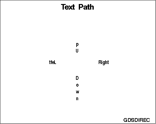
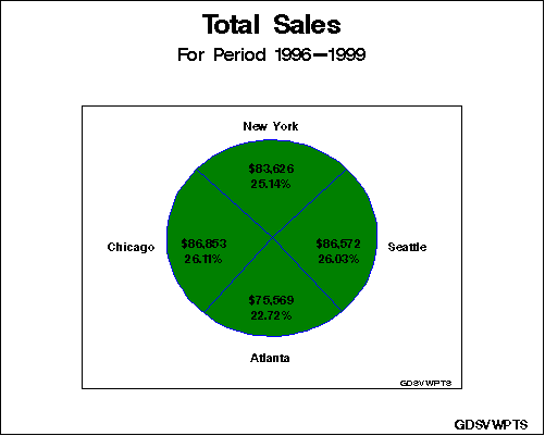
Using Viewports in DSGI
This example uses
the GCHART procedure to generate a graph, defines a viewport in which
to display it, and inserts the GCHART graph into the graphics output
being created by DSGI. Pie Chart Produced with the GCHART Procedure shows the pie chart created by the GCHART procedure. Pie Chart Inserted into DSGI Graph by Using a Viewport shows the same pie chart after it has been inserted into
a DSGI graph.
  /* set the graphics environment */
goptions reset=global gunit=pct border
     ftext=swissb htitle=6 htext=4
     colors=(black blue green red)
     hsize=7 in vsize=7 in
     targetdevice=pscolor;


  /* create data set TOTALS */
data totals;
  length dept $ 7 site $ 8;
  do year=1996 to 1999;
   do dept="Parts","Repairs","Tools";
     do site="New York","Atlanta","Chicago","Seattle";
      sales=ranuni(97531)*10000+2000;
      output;
     end;
   end;
  end;
run;

  /* define the footnote */
footnote1 h=3 j=r "GDSVWPTS ";

  /* generate pie chart from TOTALS */
  /* and create catalog entry PIE  */
proc gchart data=totals;
  format sales dollar8.;
  pie site
    / type=sum
     sumvar=sales
     midpoints="New York" "Chicago" "Atlanta" "Seattle"
     fill=solid
     cfill=green
     coutline=blue
     angle=45
     percent=inside
     value=inside
     slice=outside
     noheading
     name="GDSVWPTS";
run;

  /* define the titles */
title1 "Total Sales";
title2 "For Period 1996-1999";

  /* execute DATA step with DSGI */
data piein;

   /* prepare
SAS/GRAPH software */
   /* to accept DSGI statements */
  rc=ginit();
  rc=graph("clear");

   /* define and activate viewport for inserted graph */
  rc=gset("viewport", 1, .15, .05, .85, .90);
  rc=gset("window", 1, 0, 0, 100, 100);
  rc=gset("transno", 1);

   /* insert graph created from GCHART procedure */
  rc=graph("insert", "GDSVWPTS");

   /* display graph and end DSGI */
  rc=graph("update");
  rc=gterm();
run;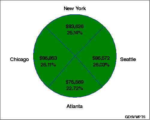
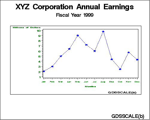
Scaling Graphs by Using Windows
This example uses the
GPLOT procedure to generate a plot of AMOUNT*MONTH and store the graph
in a permanent catalog. DSGI then scales the graph by defining a window
in another DSGI graph and inserting the GPLOT graph into that window. Plot Produced with the GPLOT Procedure shows the plot as it is displayed with the GPLOT procedure. Plot Scaled by Using a Window in DSGI shows how the same plot is displayed when the x axis is scaled from 15 to 95 and the y axis is scaled from 15 to 75.
  /* set the graphics environment */
goptions reset=global gunit=pct border
     ftext=swissb htitle=6 htext=3
     colors=(black blue green red)
     hsize=7 in vsize=5 in
     targetdevice=pscolor;

  /* create data set EARN, which holds month */
  /* and amount of earnings for that month  */
data earn;
  input month amount;
  datalines;
1 2.1
2 3
3 5
4 6.4
5 9
6 7.2
7 6
8 9.8
9 4.4
10 2.5
11 5.75
12 4.35
;
run;

  /* define the footnote for the first graph */
footnote1 j=r "GDSSCALE(a) ";

  /* define axis and symbol characteristics */
axis1 label=(color=green "Millions of Dollars")
   order=(1 to 10 by 1)
   value=(color=green);
axis2 label=(color=green "Months")
   order=(1 to 12 by 1)
   value=(color=green Tick=1 "Jan" Tick=2 "Feb" Tick=3 "Mar"
       Tick=4 "Apr" Tick=5 "May" Tick=6 "Jun"
       Tick=7 "Jul" Tick=8 "Aug" Tick=9 "Sep"
       Tick=10 "Oct" Tick=11 "Nov" Tick=12 "Dec");

symbol value=M font=special height=8 interpol=join
    color=blue width=3;

  /* generate a plot of AMOUNT * MONTH,     */
  /* and store in member GDSSCALE         */
proc gplot data=earn;
  plot amount*month
    / haxis=axis2
     vaxis=axis1
     name="GDSSCALE";
run;

  /* define the footnote and titles for    */
  /* second graph, scales the output */
footnote1 j=r "GDSSCALE(b) ";
title1 "XYZ Corporation Annual Earnings";
title2 h=4 "Fiscal Year 1999";

  /* execute DATA step with DSGI using */
  /* catalog entry created in previous */
  /* plot, but do not create a data set */
  /* (determined by specifying _NULL_) */
data _null_;

   /* prepare
SAS/GRAPH software */
   /* to accept DSGI statements */
  rc=ginit();
  rc=graph("clear");

   /* define viewport and window for inserted graph */
  rc=gset("viewport", 1, .20, .30, .90, .75);
  rc=gset("window", 1, 15, 15, 95, 75);
  rc=gset("transno", 1);

   /* insert graph previously created */
  rc=graph("insert", "GDSSCALE");

   /* display graph and end DSGI */
  rc=graph("update");
  rc=gterm();
run;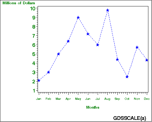
One feature not explained
in previous examples is described here:
-
The GSET(“WINDOW”, . . . ) function scales the plot with respect to the viewport that is defined. The x axis is scaled from 15 to 95, and the y axis is scaled from 15 to 75. If no viewport were explicitly defined, the window coordinates would be mapped to the default viewport, the entire graphics output area.
Enlarging an Area of a Graph by Using Windows
This example illustrates
how you can enlarge a section of a graph by using windows. In the
first DATA step, the program statements generate graphics output that
contains four pie charts. The second DATA step defines a window that
enlarges the bottom left quadrant of the graphics output and inserts
“GDSENLAR” into that window. The following program statements
produce Four Pie Charts Generated with DSGI from the first DATA step, and Area of the Graph Enlarged by Using Windows from the second DATA step:
  /* set the graphics environment */
goptions reset=global gunit=pct border
     ftext=swissb htext=3
     colors=(black blue green red)
     hsize=7 in vsize=5 in
     targetdevice=pscolor;

  /* define the footnote for the first graph */
footnote1 j=r "GDSENLAR(a) ";

  /* execute DATA step with DSGI */
data plot;

   /* prepare
SAS/GRAPH software */
   /* to accept DSGI statements */
  rc=ginit();
  rc=graph("clear", "GDSENLAR");

   /* define and draw first pie chart */
  rc=gset("filcolor", 4);
  rc=gset("filtype", "solid");
  rc=gdraw("pie", 30, 75, 22, 0, 360);

   /* define and draw second pie chart */
  rc=gset("filcolor", 1);
  rc=gset("filtype", "solid");
  rc=gdraw("pie", 30, 25, 22, 0, 360);

   /* define and draw third pie chart */
  rc=gset("filcolor", 3);
  rc=gset("filtype", "solid");
  rc=gdraw("pie", 90, 75, 22, 0, 360);

   /* define and draw fourth pie chart */
  rc=gset("filcolor", 2);
  rc=gset("filtype", "solid");
  rc=gdraw("pie", 90, 25, 22, 0, 360);

   /* display graph and end DSGI */
  rc=graph("update");
  rc=gterm();
run;

  /* define the footnote for the second graph */
footnote1 j=r "GDSENLAR(b) ";

  /* execute DATA step with DSGI  */
  /* that zooms in on a section of */
  /* the previous graph      */
data zoom;

   /* prepare
SAS/GRAPH software */
   /* to accept DSGI statements */
  rc=ginit();
  rc=graph("clear");

   /* define and activate a window   */
   /* that enlarges the lower left */
   /* quadrant of the graph      */
  rc=gset("window", 1, 0, 0, 50, 50);
  rc=gset("transno", 1);

   /* insert the previous graph into */
   /* window 1            */
  rc=graph("insert", "GDSENLAR");

   /* display graph and end DSGI */
  rc=graph("update");
  rc=gterm();
run;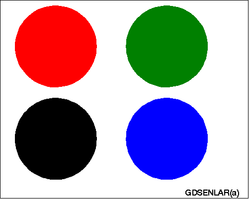
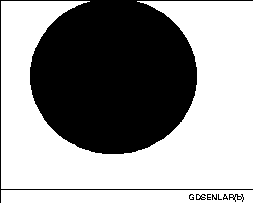
Features not explained
in previous examples are described here:
-
The GSET(“WINDOW”, . . . ) function defines a window into which the graph is inserted. In this example, no viewport is defined, so the window coordinates map to the default viewport, which is the entire graphics output area. The result of using the default viewport is that only the portion of the graph enclosed by the coordinates of the window is displayed.
Using GASK Routines in DSGI
This example illustrates
how to invoke GASK routines and how to display the returned values
in the SAS log and write them to a data set. This example assigns
a predefined color to color index 2 and then invokes a GASK routine
to get the name of the color associated with color index 2. The value
returned from the GASK call is displayed in the log and written to
a data set. Checking the Color Associated with a Particular Color Index shows how the value appears in the log. Writing the Value of an Attribute to a Data Set shows how the value appears in the data set in the OUTPUT
window.
/* execute DATA step with DSGI */ data routine; /* declare character variables used */ /* in GASK subroutines */ length color $ 8; /* preparesoftware */ /* to accept DSGI statements */ rc=ginit(); rc=graph("clear"); /* set color for color index 2 */ rc=gset("colrep", 2, "orange"); /* check color associated with color index 2 and */ /* display the value in the LOG window */ call gask("colrep", 2, color, rc); put "Current FILCOLOR =" color; output; /* end DSGI */ rc=graph("update"); rc=gterm(); run; /* display the contents of ROUTINE */ proc print data=routine; run; SAS/GRAPH
Checking the Color Associated with a Particular Color Index
3 /* execute DATA step with DSGI */ 4 data routine; 5 6 /* declare character variables used */ 7 /* in GASK subroutines */ 8 length color $ 8; 9 10 /* preparesoftware */ 11 /* to accept DSGI statements */ 12 rc=ginit(); 13 rc=graph("clear"); 14 15 /* set color for color index 2 */ 16 rc=gset("colrep", 2, "orange"); 17 18 /* check color associated with color index 2 and */ 19 /* display the value in the LOG window */ 20 call gask("colrep", 2, color, rc); 21 put "Current FILCOLOR =" color; 22 output; 23 24 /* end DSGI */ 25 rc=graph("update"); 26 rc=gterm(); 27 run; Current FILCOLOR =ORANGE SAS/GRAPH
Writing the Value of an Attribute to a Data Set
The SAS System             13:50 Tuesday, December 22, 1998   1

   Obs    color     rc

    1     ORANGE     0