SYMBOL Statement

Optional Arguments

BWIDTH=box-width

specifies the width of the box generated by either the INTERPOL=BOX or INTERPOL=HILOB option. Box-width can be any number greater than 0. By default, the value of box-width is the same as the value of the WIDTH= option, whose default value is 1. Therefore, if you specify a WIDTH= value for the line thickness of interpolated lines, and omit the BWIDTH= option, the width of the box changes according to the WIDTH= value.

Example:Creating and Modifying Box Plots

CI=line-color|_style_

specifies a color for an interpolation line (GPLOT and GBARLINE) or a contour line (GCONTOUR). The _STYLE_ value specifies the appropriate color based on the current style. If you omit the CI= option but specify the CV= option, the CI= option assumes the value of the CV= option. In this case, the CI= and CV= options specify the same color, which is the same as specifying the COLOR= option alone.

If you omit the CI= option, the color specification is searched for in this order:

1. the COLOR= option
2. the CV= option
3. the CSYMBOL= option in a GOPTIONS statement
4. each color in the color list sequentially before the next SYMBOL definition is used

See:Using Color

Example:Ordering Axis Tick Marks with SAS Date Values

CO=color

specifies a color for the following:

• outlines of filled areas generated by the INTERPOL=map/plot-pattern option
• confidence limit lines generated by the INTERPOL=R series option
• staffs, boxes, and bars generated by the high-low interpolation methods: INTERPOL=HILO, INTERPOL=BOX, and INTERPOL=STD

If you omit the CO= option, the search order for a color specification depends on the interpolation method being used.

See:Using Color

Examples:Filling the Area between Plot Lines

Creating and Modifying Box Plots

COLOR=symbol-color | _style_

specifies a color for the entire definition, unless it is followed by a more explicit specification. For the GPLOT and GBARLINE procedures, this includes plot symbols, the plot line, confidence limit lines, and outlines. For the GCONTOUR procedure, this includes contour lines and labels. The _STYLE_ value specifies the appropriate color from the current style.

Using the COLOR= option is exactly the same as specifying the same color for both the CI= and CV= options.

If COLOR= precedes the CI= or CV= option in the same statement, the CI= or CV= option is used instead.

If you do not use the COLOR=, CI=, CV=, or CO= option, the color specification is searched for in this order:

1. the CSYMBOL= option in a GOPTIONS statement
2. each color in the color list sequentially before the next SYMBOL definition is used.

Alias:C=

Style reference:Color attribute of the GraphLabelText style element

Restriction:Partially supported by Java and ActiveX

Notes:Neither the Java applet nor the ActiveX control supports using COLOR= with PROC GCONTOUR.

If you do not use a SYMBOL statement to specify a color for each symbol, but you do specify a color list in a GOPTIONS statement, then Java and ActiveX assign symbols and symbol colors differently than other devices. To ensure consistency on all devices, you should use SYMBOL statements to explicitly specify the symbols and symbol colors that you want to use in your plot.

See:Using Color

CV=value-color|_style_

specifies a color for the following:

• plot symbols in the GPLOT procedure
• the filled areas generated by the INTERPOL=map/plot-pattern option
• contour labels in the GCONTOUR procedure

The _STYLE_ value specifies the appropriate color based on the current style. If you omit the CV= option but specify the CI=, the CV= option assumes the value of the CI= option. In this case, the CV= and CI= options specify the same color, which is the same as specifying the COLOR= option alone.

If you omit the CV= option, the color specification is searched for in this order:

1. the COLOR= option
2. the CI= option
3. the CSYMBOL= option in a GOPTIONS statement
4. each color in the color list sequentially before the next SYMBOL definition is used

Restriction:Partially supported by Java and ActiveX

Note:Neither the Java applet nor the ActiveX control supports using the CV= option with PROC GCONTOUR.

See:Using Color

Examples:Ordering Axis Tick Marks with SAS Date Values

Creating and Modifying Box Plots

Filling the Area between Plot Lines

FONT=“font”

specifies the font for the plot symbol (GPLOT, GBARLINE) or contour labels (GCONTOUR) specified by the VALUE= option. The font specification must be enclosed in quotation marks and can include the /bold and /italic font modifiers.

By default, the symbol specified by the VALUE= option is taken from the special symbol table shown in Special Symbols for Plotting Data Points. To use symbols from the special symbol table, you must omit the FONT= option.

To use a symbol that is not in that special symbol table, specify the font containing the symbol and the character code or hexadecimal code of the symbol that you want to use. You can also specify text instead of special symbols. For example:

symbol font="Albany AMT" value="80"x;   /* hexadecimal code for the Euro symbol */
symbol font="Monotype Sorts" value="s";   /* character code for a filled triangle */
symbol font="Cumberland AMT/bo" value="F";   /* prints the letter F in bold */

To cancel a font specification and return to the default special symbol table, enter a null font specification:

symbol font= value=dot;

Alias:F=

Restrictions:Not supported by Java and ActiveX

Only single-byte symbol characters are supported.

Note:If the font is specified with the Unicode attribute,: then the font symbol values are processed as double-byte characters. Double-byte characters resolve to question marks.

See: VALUE=special-symbol | text-string | SPECIAL | NONE

Specifying Plot Symbols

Specifying Special Characters Using Character and Hexadecimal Codes

Example:Labeling Contour Lines, Modifying the Horizontal Axis, Modifying the Legend

HEIGHT=symbol-height<units>

specifies the height in number of units of plot symbols (GPLOT, GBARLINE) or contour labels (GCONTOUR).

Alias: H=

Restriction:Partially supported by Java and ActiveX

Notes:With the Java device driver, the minimum height is two pixels; with ActiveX a symbol can be so small as to be invisible.

Neither the Java applet nor the ActiveX control supports HEIGHT= with PROC GCONTOUR.

The HEIGHT= option affects only the height of the symbols and labels on the plot; it does not affect the height of any symbols that might appear in a legend.

The HEIGHT option overrides the MarkerSize attribute in ODStyles. For more information about ODS styles, see the SAS Output Delivery System: User's Guide.

See: the option SHAPE=BAR(width<units>,height<units>) <units> | LINE(length) <units> | SYMBOL(width<units>,height<units>) <units> in the LEGEND statement

Examples:Creating and Modifying Box Plots

Rotating Plot Symbols through the Color List

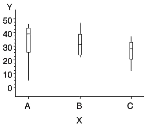
INTERPOL=BOX<option(s)><00...25>

produces box-and-whisker plots. The bottom and top edges of the box are located at the sample 25th and 75th percentiles. The center horizontal line is drawn at the 50th percentile (median). By default, INTERPOL=BOX. In this case the vertical lines, or whiskers, are drawn from the box to the most extreme point less than or equal to 1.5 interquartile ranges. (An interquartile range is the distance between the 25th and the 75th sample percentiles.) Any value more extreme than this is marked with a plot symbol.

Values for option(s) are one or more of these:

F

fills the box with the color specified by CV= and outlines the box with the color specified by CO=

J

joins the median points of the boxes with a line

T

draws tops and bottoms on the whiskers.

In addition, you can specify a percentile to control the length of the whiskers within the range 00 through 25. These are examples of percentile specifications and their effect:

00

specifies high or low extremes. INTERPOL=BOX00 is not the same as the default, INTERPOL=BOX.

01

specifies 1st percentile low, 99th high.

05

specifies 5th percentile low, 95th high.

10

specifies 10th percentile low, 90th high.

25

specifies 25th percentile low, 75th high. Since the box extends from the 25th to the 75th percentile, no whiskers are produced.

Box Plot shows the type of plot INTERPOL=BOX produces.

Box Plot

You cannot use the GPLOT procedure PLOT statement option AREAS= with INTERPOL=BOX.

To increase the thickness of all box plot lines, including the box, whiskers, join line, and top and bottom ticks, use the WIDTH= option.

To increase the width of the box itself, use the BWIDTH= option. By default the value of the BWIDTH= option is the same as the value of the WIDTH= option. Therefore, if you specify a value for the WIDTH= option and omit the BWIDTH= option, the width of the box changes.

For a scatter effect with the box, use a multiple plot request, as in this example:

symbol1 i=none v=star color=green;
symbol2 i=box v=none color=blue;
proc gplot data=test;
   plot (y y)*x / overlay;

Alias: I=

Notes:If you use the HAXIS= or VAXIS= options in the PLOT statement or the ORDER= option in an AXIS definition to restrict the range of axis values, by default any observations that fall outside the axis range are excluded from the interpolation calculation. See the MODE=EXCLUDE | INCLUDE.

When using DEVICE=JAVA and DEVICE=JAVAIMG with overlaid plots, different interpolations are supported per overlay unless any of the interpolations is BOX, HILO or STD. When any of these interpolations are encountered, the first interpolation specified becomes the only interpolation that is used for all overlays. All other interpolations are ignored.

Example:Creating and Modifying Box Plots

INTERPOL=HILO<C><option>

specifies that a solid vertical line connect the minimum and maximum Y values for each X value. The data should have at least two values of Y for every value of X. Otherwise, the single value is displayed without the vertical line.

By default, for each X value, the mean Y value is marked with a tick. This is shown in High-Low Plot.

To specify high, low, close stock market data, include this option:

C

draws tick marks at the close value instead of at the mean value. Specifying C assumes that there are three values of Y (HIGH, LOW, and CLOSE) for every value of X. If more or fewer than three Y values are specified, the mean is ticked. The Y values can be in any order in the input data set.

In addition, you can specify one of these values for option:

B

connects the minimum and maximum Y values with bars instead of lines. Use the BWIDTH= option to increase the width of the bars.

J

joins the mean values or the close values (if HILOC is specified) with a line. This point is not marked with a tick mark. You cannot use the PLOT statement option AREAS= with INTERPOL=HILOJ.

T

adds tops and bottoms to each line.

BJ

connects maximum and minimum values with a bar and joins the mean or close values.

TJ

adds tops and bottoms to the lines and joins the mean or close values.

High-Low Plot shows the type of plot INTERPOL=HILO produces. Plot symbols in the form of dots have been added to this figure.

High-Low Plot

To increase the thickness of all lines generated by the INTERPOL=HILO option, use the WIDTH= option.

When using DEVICE=JAVA and DEVICE=JAVAIMG with overlaid plots, different interpolations are supported per overlay unless any of the interpolations is BOX, HILO or STD. When any of these interpolations are encountered, the first interpolation specified becomes the only interpolation that is used for all overlays. All other interpolations are ignored.

Alias: I=

Restriction: Partially supported by Java

Note:If you use the HAXIS= or VAXIS= options in the PLOT statement or the ORDER= option in an AXIS definition to restrict the range of axis values, by default any observations that fall outside the axis range are excluded from the interpolation calculation. See the option MODE=EXCLUDE | INCLUDE .

Example:Ordering Axis Tick Marks with SAS Date Values

INTERPOL=JOIN

connects data points with straight lines. Points are connected in the order in which they occur in the input data set. Therefore, the data should be sorted by the independent (horizontal axis) variable.

If the data contain missing values, the observations are omitted. However, the plot line is not broken at missing values unless the SKIPMISS option is used.

Alias:I=

See:SKIPMISS

Missing Values

INTERPOL=L<degree><P><S>

specifies a Lagrange interpolation to smooth the plot line. Specify one of these values for degree:

1 | 3 | 5

specifies the degree of the Lagrange interpolation polynomial. By default, degree is 1.

In addition, you can specify one or both of these:

P

specifies a parametric interpolation.

S

sorts a data set by the independent variable before plotting its data.

The Lagrange methods are useful chiefly when data consist of tabulated, precise values. A polynomial of the specified degree (1, 3, or 5) is fitted through the nearest 2, 4, or 6 points. In general, the first derivative is not continuous. If the values of the horizontal variable are not strictly increasing, the corresponding parametric method (L1P, L3P, or L5P) is used.

Specifying INTERPOL=L1P, INTERPOL=L3P, or INTERPOL=L5P results in a parametric Lagrange interpolation of degree 1, 3, or 5, respectively. Both the horizontal and vertical variables are processed with the Lagrange method and a parametric interpolation of degree 1, 3, or 5, using the distance between points as a parameter.

Alias:I=

INTERPOL=map/plot-pattern

specifies that a pattern fill the polygon that has been defined by the data points. Values for map/plot-pattern are as follows:

MEMPTY

specifies an empty pattern. EMPTY and E are valid aliases.

The Java applet does not support this option.

Alias:ME

MSOLID

specifies a solid pattern. SOLID and S are valid aliases

Alias:MS

Mdensity<style<angle>>

specifies a shaded pattern. (The Java applet does not support this option.)

Density specifies the density of the pattern's shading. Specify a number from 1 to 5. The number 1 produces the lightest shading and 5 produces the heaviest.

Style specifies the direction of pattern lines:

N

specifies parallel lines (the default)

X

specifies crosshatched lines.

Angle specifies the starting angle for parallel or crosshatched lines. Specify a number from 0 to 360. The number specifies the degree at which the parallel lines are drawn. By default, angle is 0 (lines are parallel to the horizontal axis).

The INTERPOL=map/plot-pattern option only works if the data are structured so that the data points and, consequently, the plot lines form an enclosed area. The plot lines should not cross each other.

Alias:I=

Restriction:Partially supported by Java

See:PATTERN Statement

Example:Filling the Area between Plot Lines

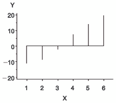
INTERPOL=NEEDLE

draws a vertical line from each data point to a horizontal line at the 0 value on the vertical axis or the minimum value on the vertical axis. The horizontal line is drawn automatically.

Needle Plot shows the type of plot INTERPOL=NEEDLE produces. Plot symbols are not displayed in this figure.

Needle Plot

You cannot use the PLOT statement option AREAS= with INTERPOL=NEEDLE.

Alias:I=

INTERPOL=NONE

suppresses any interpolation and, if the VALUE= option is not specified, also suppresses plot points. If no interpolation method is specified in a SYMBOL statement and if the graphics option INTERPOL= is not used, INTERPOL=NONE is the default.

You cannot use the PLOT statement option AREAS= with INTERPOL=NONE.

Alias:I=

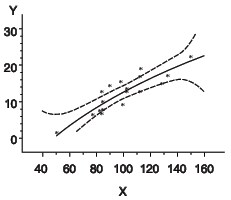
INTERPOL=R<type><0><CLM | CLI<50...99>>

specifies that a plot is a regression analysis. By default, the regression type is L, regression lines are not forced through plot origins, and confidence limits are not displayed.

The regression line is drawn in the line type specified in the LINE= option. By default, the line type of the regression line is 1.

Type indicates the type of regression. Specify one of these values for type:

L

requests linear regression representing the regression equation

Y= β ₀ + β ₁ X.

Q

requests quadratic regression representing the regression equation

Y= β ₀ + β ₁ X + β ₂ X².

C

requests cubic regression representing the regression equation

Y= β ₀ + β ₁ X+ β ₂ X ² + β ₃ X³.

Note: When least-square solutions for the parameters are not unique, most devices use a quadratic equation by default for the interpolation. However, the Java and ActiveX device drivers might pick a cubic solution to use.

CAUTION:

You must specify type if you use 0, or CLI, or CLM, in order to achieve the expected results.

For example, the following interpolation request is correct:

I=RL0CLM95

while the following interpolation request is incorrect because type is missing although 0 is specified:

I=R0CLM95

and the following interpolation request is incorrect because type is missing although CLM is indicated:

I=RCLM95

To force the regression line through a (0,0) origin, specify the following:

0

eliminates the β ₀ parameter, or intercept, from the regression equation. If the origin is at (0,0), also forces the regression line through the origin. For example, if you specify 0 for a linear regression, the plot line represents the equation

Y= β₁ X.

Note: To force the regression line through the origin (0,0) when the data ranges do not place the origin at (0,0), use the GPLOT procedure options HZERO and VZERO (ignored if the data contain negative values), or use the HAXIS= and VAXIS= options to specify axes ranges from 0 to maximum data value. If the data ranges contain negative values and the HAXIS= and VAXIS= options specify ranges starting at 0, only values within the displayed range are used in the interpolation calculations.

To display confidence limits, specify one of these:

CLM

displays confidence limits for mean predicted values.

CLI

displays confidence limits for individual predicted values.

You can specify confidence levels from 50% to 99%. By default, the confidence level is 95%. Include a confidence level specification only if you use CLM or CLI.

The line type used for the confidence limit lines is determined by adding 1 to the values of LINE=. By default, the line type of confidence limit lines is 2.

Plot of Regression Analysis and Confidence Limits shows the type of plot INTERPOL=RCCLM95 produces (cubic regression analysis with 95% confidence limits).

Plot of Regression Analysis and Confidence Limits

Alias:I=

Restriction:Partially supported by Java

Example:Plotting Two Variables

INTERPOL=SM<nn><P><S>

specifies that a smooth line is fit to data using a spline routine. INTERPOL=SM is a method for smoothing noisy data. The points on the plot do not necessarily fall on the line.

The relative importance of plot values versus smoothness is controlled by nn. Values for nn are as follows:

0...99

produces a cubic spline that minimizes a linear combination of the sum of squares of the residuals of fit and the integral of the square of the second derivative(footnote1). The greater the nn value, the smoother the fitted curve. By default, the value of nn is 0.

In addition, specify one or both of these:

P

specifies a parametric cubic spline.

S

sorts data by the independent variable before plotting.

Alias:I=

Restriction:Not supported by Java

INTERPOL=SPLINE<P><S>

specifies that the interpolation for the plot line use a spline routine. INTERPOL=SPLINE produces the smoothest line and is the most efficient of the nontrivial spline interpolation methods.

Spline interpolation smooths a plot line using a cubic spline method with continuous second derivatives(footnote2) This method uses a piecewise third-degree polynomial for each set of two adjacent points. The polynomial passes through the plotted points and matches the first and second derivatives of neighboring segments at the points.

Specify one or both of these:

P

specifies a parametric spline interpolation method. This interpolation uses a parametric spline method with continuous second derivatives. Using the method described earlier for the spline interpolation, a parametric spline is fitted to both the horizontal and vertical values. The parameter used is the distance between points

If two points are so close together that the computations overflow, the second point is not used.

S

sorts a data set by the independent variable before plotting its data.

Alias:I=

Notes:When points on the graph are out of range of the axis values, the curve is clipped. If an end point is out of range, no curve is drawn. Out-of-range conditions can be caused by restricting the range of axis values with the HAXIS= or VAXIS= option in the PLOT statement or the ORDER= option in an AXIS definition.

When points on the graph are close together and a spline interpolation is used, the Java applet is unable to draw some line types correctly.

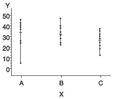
INTERPOL=STD<1 | 2 | 3><variance><option(s)>

specifies that a solid line connect the mean Y value with ± 1, 2, or 3 standard deviations for each X. The sample variance is computed about each mean, and from it, the standard deviation s_y is computed. Variance can be one or both of these:

M

computes .

P

computes sample variances using a pooled estimate, as in a one-way ANOVA model.

In addition, specify one of these values for option(s):

B

connects the minimum and maximum Y values with bars instead of lines.

J

connects the means from bar to bar with a line.

T

adds tops and bottoms to each line.

BJ

connects maximum and minimum values with a bar and joins the mean values.

TJ

adds tops and bottoms to the lines and joins the mean values.

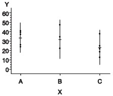
Plot of Standard Deviations shows the type of plot INTERPOL=STD produces. A horizontal tick is drawn at the mean. Plot symbols in the form of dots have been added to this figure.

Plot of Standard Deviations

If you restrict the range of axis values by using the HAXIS= or VAXIS= option in a PLOT statement or the ORDER= option in an AXIS definition, by default any observations that fall outside the axis range are excluded from the interpolation calculation. See the MODE=EXCLUDE | INCLUDE.

To increase the thickness of all lines generated by the INTERPOL=STD option, use the WIDTH= option.

You cannot use the PLOT statement option AREAS= with INTERPOL=STD.

When using DEVICE=JAVA and DEVICE=JAVAIMG with overlaid plots, different interpolations are supported per overlay unless any of the interpolations is BOX, HILO or STD. When any of these interpolations are encountered, the first interpolation specified becomes the only interpolation that is used for all overlays. All other interpolations are ignored.

Alias:I=

Restriction:Partially supported by Java

Notes:By default, two standard deviations are used.

By default, the vertical axis ranges from the minimum to the maximum Y value in the data. If the requested number of standard deviations from the mean covers a range of values that exceeds the maximum or is less than the minimum, the STD lines are cut off at the minimum and maximum Y values. When this cutoff occurs, rescale the axis using VAXIS= in the PLOT statement or ORDER= in an AXIS definition so that the STD lines are shown.

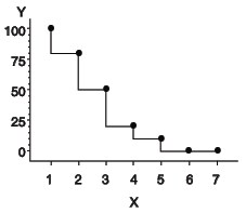
INTERPOL=STEP<placement><J><S>

specifies that the data are plotted with a step function. By default, the data point is on the left of the step, the steps are not joined with a vertical line, and the data are not sorted before processing.

Specify one of these values for placement:

L

displays the data point on the left of the step.

R

displays the data point on the right of the step.

C

displays the data point in the center of the step.

In addition, specify one or both of these:

J

produces steps joined with a vertical line.

S

sorts unordered data by the independent variable before plotting.

Step Plot shows the type of plot that INTERPOL=STEPJR produces. Plot symbols in the form of dots have been added to this figure.

Step Plot

Alias:I=

Notes:When a step is retraced in order to locate its center point, the GIF, JPEG, PNG, ACTXIMG, Java, and JAVAIMG devices treat this as effectively not drawing that part of the step at all. ActiveX, however, draws each part of the step, which results in a somewhat different graph.

The ActiveX and Java devices do not support the S option. For these devices, use the SORT procedure or the ORDER= option on an AXIS statement to sort your data by the independent variable before calling the GPLOT or GBARLINE procedure.

LINE=line-type

specifies the line type of the plot line in the GPLOT procedure, or the contour line in the GCONTOUR procedure:

1

specifies a solid line.

2...46

specifies a dashed line.

Line types are shown in Line Types. By default, LINE=1.

Alias:L=

Restriction:Partially supported by Java and ActiveX

Notes:This option overrides the LineStyle attribute in graph styles.

Neither the Java applet nor ActiveX control supports GCONTOUR.

MODE=EXCLUDE | INCLUDE

specifies that any interpolation method exclude or include data values that are outside the range of plot axes. By default, MODE=EXCLUDE prevents values outside the axis range from being displayed.

If you control the range of values displayed on an axis by using HAXIS= and VAXIS= in the GPLOT procedure, or ORDER= in an AXIS definition, any data points that lie outside the range of the axes are discarded before interpolation is applied to the data. Using these options to control value ranges has a particularly noticeable effect on the high-low interpolation methods, which include INTERPOL=HILO, INTERPOL=BOX, and INTERPOL=STD. Regression analysis also represents only part of the original data.

Restriction:Not supported by Java and partially supported by ActiveX

See:Values Out of Range

POINTLABEL<=(label-description(s)) | NONE>

labels plot points. The labels always use the format that is assigned to the variable or variables whose values are used for the labels. POINTLABEL without any specified descriptions labels points with the Y value. NONE suppresses the point labels. Label-description(s) can be used to change the variable whose values are used to label points, and to change features of the label text, such as the color, font, or size of the text.

Label-description(s) can be one or more of these:

COLOR=text-color

specifies the color of the label text. The default is the first color from the color list.

Alias:C=

Note:If you do not specify a color on a SYMBOL statement, the symbol definition is rotated through the color list before the next SYMBOL statement is used. Thus, if your plot contains multiple plot lines and you want to limit your POINTLABEL specification to a single line, you must specify a color in the SYMBOL statement that contains the POINTLABEL description.

DROPCOLLISIONS | NODROPCOLLISIONS

specify DROPCOLLISIONS to drop new labels if they collide with a label already in use. Specify NODROPCOLLISIONS to retain all labels. The default is DROPCOLLISIONS.

The algorithm for the placement of markers tries to avoid placing labels such that they collide. If the algorithm is unable to avoid a collision, then the default DROPCOLLISIONS is to drop the new label, whereas NODROPCOLLISIONS retains even colliding labels.

FONT=font | NONE

specifies the font for the text. See Specifying Fonts in SAS/GRAPH Programs for details about specifying font. If you omit FONT=, a font specification is searched for in this order:

1. the FTEXT= option in a GOPTIONS statement
2. the default hardware font, NONE

Alias:F=

Restriction:Only single-byte symbol characters are supported.

Note:If the font is specified with the Unicode attribute, then the font symbol values are processed as double-byte characters. Double-byte characters resolve to question marks. POINTLABEL specifications that mix double- and single-byte characters are processed as if the entire string consists of double-byte characters.

HEIGHT=text-height <units >

specifies the height of the text characters in number of units. By default, HEIGHT=1 CELL. If you omit HEIGHT=, a text height specification is searched for in this order:

1. the HTEXT= option in a GOPTIONS statement
2. the default value, 1

Alias:H=

JUSTIFY=CENTER | LEFT | RIGHT

specifies the horizontal alignment of the label text. The default is CENTER. The location of the point label is relative to the location of the corresponding data point.

Alias:J=C | L | R

POSITION=TOP | MIDDLE | BOTTOM

specifies the vertical placement of the label text. The default is TOP. The location of the point label is relative to the location of the corresponding data point.

“#var1<:#var2 <$char>>”

specifies the variable or variables whose values label the plot points, and the delimiter between more than one variable. The variable specification must be enclosed in either single or double quotation marks. The first specified variable must be prefixed with a pound sign (#). If a second variable is specified, it must be prefixed with a colon and a pound sign (:#). When you specify two variables, you can also specify the character to display as the delimiter between variable values in the plot label.

By default, if the POINTLABEL= option is specified without naming a label variable, the Y values label the plot points. You can change the default by using “#var” to specify a different variable whose values should label the points. For example, you might specify the name of the X variable. The following option specifies the variable SALES as the variable whose values label plot points:

POINTLABEL=("#sales")

Alternatively, you can label the plot points with the values of two variables, in either order. The order in which you specify the variables determines the order that the values are displayed in the label. The following option specifies variables HEIGHT and WEIGHT; which in the label displays the value for HEIGHT and then the value for WEIGHT:

POINTLABEL=("#height:#weight")

anksBy default, when you specify two variables, a colon (:) is displayed in the label to separate the variable values. To change the character that displays as the delimiter, use the $ syntax to specify an alternative character. The following option specifies a vertical bar (|) as the delimiter in the label:

POINTLABEL=("#height:#weight $|")

The $ syntax must be within the same quotation marks as the variable specification. The $ specification can precede or follow the variable specification, but it must be separated from the variable specification by at least one space.

Specify as many label-description suboptions as you want. Enclose them all within a single set of parentheses, and separate each suboption from the others by at least one space.

Restrictions:When creating output using the JAVA or ACTIVEX devices, the variables that you specify must be for the plot’s X and Y variables. Specifying any other variables causes unexpected labeling.

There is a 16-character length limit for each variable. A maximum character length limit of thirty-three characters is possible. This can be composed of X and Y variables, any other valid data set variable, and a separator as required.

Notes:Specifying a delimiting character with the $ only changes the character that is displayed in the label. It does not change the syntax of the variable specification, which requires a colon and pound sign (:#) to precede the second variable.

Creating multiple plots that share the same or close-ranging data points, along with specifying appearance suboptions, can result in multiple data point labels.

Depending on the appearance suboptions, for example HEIGHT=, that you use for point labels, the labels can overlap other elements on the graph. When this occurs a warning appears in the SAS log.

The algorithm for placing markers on the graph repositions point labels that are overwriting a graphics output area boundary. When this occurs a note appears in the SAS log.

REPEAT=number-of-times

specifies the number of times that a SYMBOL definition is applied before the next SYMBOL definition is used. By default, REPEAT=1.

The behavior of REPEAT= depends on whether any of the SYMBOL color options (CI=, CV=, CO=, and COLOR=) or the CSYMBOL= graphics option also is used:

• If any SYMBOL color option also is used in the SYMBOL definition, that SYMBOL definition is repeated the specified number of times in the specified color.
• If no SYMBOL color option is used but the CSYMBOL= graphics option is currently in effect, the SYMBOL definition is repeated the specified number of times in the specified color.
• If no SYMBOL statement color options are used and the CSYMBOL= graphics option is not used, the SYMBOL definition is cycled through each color in the color list, and then the entire group generated by this cycle repeats the number of times specified by the REPEAT= option. Thus, the total number of iterations of the SYMBOL definition depends on the number of colors in the current color list.

  Neither the Java applet nor ActiveX control supports GCONTOUR.

Alias:R=

Restriction:Partially supported by Java and ActiveX

See:Using the SYMBOL Statement

SINGULAR=n

tunes the algorithm used to check for singularities. The default value is machine dependent but is approximately 1E-7 on most machines. This option is rarely needed.

STEP=distance<units>

specifies the minimum distance between labels on contour lines The value of distance must be greater than zero. By default, STEP=65PCT.

When you use the STEP= option, specify the minimum distance that you want between labels. The option then calculates how many labels it can fit on the contour line, taking into account the length of the labels and the minimum distance that you specified. Once it has calculated how many labels it can fit while retaining the minimum distance between them, it places the labels, evenly spaced, along the line. Consequently, the space between labels can be greater than what you specify, although it is never less.

In general, to increase the number of labels from the default, reduce the value of distance.

If the procedure cannot write the label at a particular location on the contour, for example because the contour line makes a sharp turn, the label might be placed farther along the line or omitted. If labels are omitted, a note appears in the log. Specifying a low value for the GCONTOUR procedure's TOLANGLE= option can also cause labels to be omitted. This specification forces the procedure to select smoother labeling locations, which might not be available on some contours.

Restriction:Not supported by Java and ActiveX

Note:If you specify units of PCT or CELLS, the STEP= option calculates the distance between the labels based on the width of the graphics output area, not the height. For example, if you specify STEP=50PCT and if the graphics output area is 9 inches wide, the distance specified is 4.5 inches. A value less than 10% is ignored and 10% is used instead.

Example:Labeling Contour Lines, Modifying the Horizontal Axis, Modifying the Legend

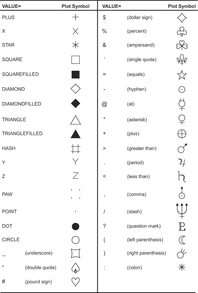
VALUE=special-symbol | text-string | SPECIAL | NONE

specifies a plot symbol for the data points (GPLOT and GBARLINE).

• If you omit the SYMBOL statement, plot points are generated using the default plot symbols. If you specify a SYMBOL statement, but do not specify the VALUE= option, the plot symbols are suppressed.
• specifies contour-label text in a contour plot (GCONTOUR). By default with the AUTOLABEL option, GCONTOUR labels contour lines with the contour variable's value at that contour level.
• VALUE=SPECIAL enables you to define unique special symbols for up to 12 plots (GPLOT) in one SYMBOL statement. Some of the symbols include the following: CIRCLE, DIAMOND, DIAMONDFILLED, DOT, DOTFILLED, HASH, PAW, POINT, PLUS, SQUARE, SQUAREFILLED, STAR, TRIANGLE, TRIANGLEFILLED, X, Y, and Z. See Special Symbols for Plotting Data Points for the complete list. This option is useful when the number of plots in your graph is variable. Rather than writing a SYMBOL statement for each possible plot, you can use VALUE=SPECIAL in one SYMBOL statement to define symbols for up to 12 individual plots.
• VALUE=NONE suppresses plot symbols at the data points, or labels on the contour lines. You can set the VALUE=NONE option independent of the INTERPOL= option.

Values for special-symbol are the names and characters shown in Special Symbols for Plotting Data Points. The special symbol table can be used only if the FONT= option is not used or a null value is specified:

font=,

This means that you cannot use VALUE=special-symbol or VALUE=SPECIAL if you are using the FONT= option.

Special Symbols for Plotting Data Points

Note: The words or special characters in the VALUE= column are entered exactly as shown.

To specify a single quotation mark, you must enclose it in double quotation marks:

value="'"

To specify a double quotation mark, you must enclose it in single quotation marks:

value='"'

In some operating environments, punctuation characters might require single quotation marks.

If you use VALUE=text-string to specify a plot symbol, you must also use the FONT= option to specify a symbol font or a text font. If you specify a symbol font, the characters in the string are character codes for the symbols in the font. If you specify a text font, the characters in the string are displayed. If you specify a text string containing quotation marks or blanks, enclose the string in single quotation marks.

For example, if you specify this statement, the plot symbol is the word “plus” instead of the symbol +:

symbol font=swiss value=plus;

Java and ActiveX support the following characters from the Marker Font for special-symbol and SPECIAL:

Marker-font Symbols Supported by Java and ActiveX

Character	Aliases
Marker	Cone, Pyramid, Default
Square	Cube
Star
Circle	Sphere, Dot, Balloon
Plus	Cross
Flag	Y
X
Prism	Z
Spade	“
Heart	#
Diamond	$
Club	%
Hexagon	Paw
Cylinder	Hash

Note: If you do not use a SYMBOL statement to specify a color for each symbol, but you do specify a color list in a GOPTIONS statement, then Java and ActiveX assign colors to symbols differently than do the other device drivers. To ensure consistency on all devices, for VALUE=special-symbol or VALUE=text-string, you should specify the desired color of each symbol. If you do not specify a symbol color, SAS/GRAPH uses the first default color and the first symbol. It uses each color in the list of default colors until the list is exhausted. SAS/GRAPH then selects the next symbol and begins again with the first default color. It rotates the new symbol through the list of default colors before selecting another symbol. It continues selecting new symbols and colors until no more symbols are needed.

For VALUE=SPECIAL, the way in which symbols and their colors are assigned is different from VALUE=special-symbol and VALUE=text-string. For VALUE=SPECIAL, when generating symbols for a plot, rather than rotating each symbol through the list of colors, SAS/GRAPH rotates through the 12 special symbols and assigns each symbol a color from the color list. The symbols and the symbol colors that are used in a plot depend on the following:

• whether a symbol color is specified in the SYMBOL statement or in the GOPTIONS statement
• the number of colors in the color list when a symbol color is not specified

Alias:V=

Restriction:Partially supported by Java and ActiveX

Notes:For ActiveX output, the VALUE= option is not supported when INTERPOL=HILO or INTERPOL=STD. You can use the OVERLAY option with GPLOT to get symbols to appear on the data points.

The VALUE option overrides the MarkerSymbol attribute in graph styles.

See:Symbol Sequences Generated from SYMBOL Statements FONT=font | NONE Specifying Plot Symbols

Examples:Rotating Plot Symbols through the Color List

Creating and Modifying Box Plots

Labeling Contour Lines, Modifying the Horizontal Axis, Modifying the Legend

WIDTH=thickness-factor

specifies the thickness of interpolated lines (GPLOT) or contour lines (GCONTOUR). thickness-factor is a number. The thickness of the line increases directly with thickness-factor. By default, WIDTH=1.

WIDTH= also affects all the lines in box plots (INTERPOL=BOX), high-low plots with bars (INTERPOL=HILOB), and standard deviation plots (INTERPOL=STD). It also affects the outlines of the area generated by the AREAS= option in the PLOT statement of the GPLOT procedure.

Alias:W=

Style reference: LineThickness attribute of the GraphAxisLines element

Restriction:Partially supported by Java and ActiveX

Notes:By default, the value specified by WIDTH= is used as the default value for the BWIDTH= option. For example, specifying WIDTH=6 also sets BWIDTH= to 6 unless you explicitly assign a value to the BWIDTH= option.

Java and ActiveX do not provide the same measure of control for width as the other SAS/GRAPH device drivers. Measurements are translated to pixels rather than a percentage. For the JAVA, JAVAIMG, ACTIVEX, and ACTXIMG devices, the maximum width is 6.

Examples:Ordering Axis Tick Marks with SAS Date Values

Creating and Modifying Box Plots