PROC PSMOOTH: Displaying Plot of PROC PSMOOTH Output Data Set

The PSMOOTH Procedure

Example 11.1 Displaying Plot of PROC PSMOOTH Output Data Set

Data other than the output data sets from the CASECONTROL and FAMILY procedures can be used in PROC PSMOOTH; here is an example of how to use $\text{[math]}$ -values from another source, read into a SAS data set by using the following DATA step.

   data tests;
      input Marker Pvalue @@;
      datalines;
    1  0.72841     2   0.40271
    3  0.32147     4   0.91616
    5  0.27377     6   0.48943
    7  0.40131     8   0.25555
    9  0.57585    10   0.20925
   11  0.01531    12   0.23306
   13  0.69397    14   0.33040
   15  0.97265    16   0.53639
   17  0.88397    18   0.03188
   19  0.13570    20   0.79138
   21  0.99467    22   0.37831
   23  0.86459    24   0.97092
   25  0.19372    26   0.85339
   27  0.32078    28   0.31806
   29  0.00655    30   0.82401
   31  0.65339    32   0.36115
   33  0.92704    34   0.49558
   35  0.64842    36   0.43606
   37  0.67060    38   0.87520
   39  0.78006    40   0.27252
   41  0.28561    42   0.80495
   43  0.98159    44   0.97030
   45  0.53831    46   0.78712
   47  0.88493    48   0.36260
   49  0.53310    50   0.65709
   51  0.26527    52   0.46860
   53  0.55465    54   0.54956
   55  0.44477    56   0.04933
   57  0.12016    58   0.76181
   59  0.80158    60   0.18244
   61  0.01382    62   0.15100
   63  0.04713    64   0.52655
   65  0.59368    66   0.94420
   67  0.60104    68   0.32848
   69  0.90195    70   0.21374
   71  0.95471    72   0.14145
   73  0.95215    74   0.70330
   75  0.19921    76   0.99086
   77  0.75736    78   0.23761
   79  0.87260    80   0.91472
   81  0.33650    82   0.26160
   83  0.41948    84   0.62817
   85  0.48721    86   0.67093
   87  0.53089    88   0.13623
   89  0.44344    90   0.41172
   ;

The following code applies Simes’ method for multiple hypothesis testing in order to adjust the $\text{[math]}$ -values.

   proc psmooth data=tests out=pnew simes bandwidth=3 to 9 by 2 neglog;
      var Pvalue;
      id Marker;
   run;
   
   proc sgplot data=pnew;
      series x=Marker y=Pvalue    / lineattrs=(pattern=solid);
      series x=Marker y=Pvalue_S3 / lineattrs=(pattern=solid);
      series x=Marker y=Pvalue_S5 / lineattrs=(pattern=solid);
      series x=Marker y=Pvalue_S7 / lineattrs=(pattern=solid);
      series x=Marker y=Pvalue_S9 / lineattrs=(pattern=solid);
      refline 3.0 / axis=y;
      discretelegend;
   run;

The NEGLOG option is used in the PROC PSMOOTH statement to facilitate plotting the $\text{[math]}$ -values by using the GPLOT procedure of SAS/GRAPH. The plot in Output 11.1.1 demonstrates the effect of the different window sizes that are implemented.

Output 11.1.1 Line Plot of Negative Log $\text{[math]}$ -Values

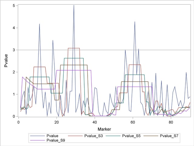
Note how the plots become progressively smoother as the window size increases. Points above the horizontal reference line represent significant $\text{[math]}$ -values at the 0.05 level. While six of the markers have significant $\text{[math]}$ -values before adjustment, only the method that uses a bandwidth of 3 finds any significant markers, all in the 26–32 region. This can be an indication that the other five markers are significant only by chance; that is, they might be false positives.

Top of Page