SELECT Statement
Retrieves columns and rows of data from tables.
| Categories: | Data Definition |
| Data Manipulation | |
| Supports: | EXECUTE Statement |
| Data source: | SAS data set, SPD Engine data set, Aster, DB2 under UNIX and PC, Greenplum, HDMD, Hive, MDS, MySQL, Netezza, ODBC, Oracle, PostgreSQL, SAP, SAP HANA, Sybase IQ, Teradata |
Syntax
[{AND | OR} [NOT] {<sql-expression> | (<search-condition>)}]}]
Details
Overview
-
A query specification begins with the SELECT keyword (called a SELECT clause) and cannot be used by itself. It reads column values from one or more tables and enables you to define conditions for the data that will be returned from the tables. It must be used as a part of another SQL statement and can return more than one row. A query specification creates a virtual table. For example:
select column(s)
from table(s)
where condition(s);
SELECT Clause
Syntax
Arguments
ALL
includes all rows, including duplicate rows in the result table.
DISTINCT
eliminates duplicate rows in the result table.
<select-list>
specifies the columns to be selected for the result table.
*
selects all columns in the table that is listed in the FROM clause.
column-alias
assigns a temporary, alternate name to the column.
column [AS column-alias]
selects a single column. When [AS column-alias] is specified, assigns the column alias to the column.
<query-specification>
specifies an embedded SELECT subquery.
| See | Overview of Subqueries |
<sql-expression> [AS column-alias]
derives a column name from an expression.
| See | <sql-expression> |
table.*
selects all columns in the table.
table-alias.*
selects all columns in the table.
| See | Table Aliases |
Asterisk (*) Notation
Column Aliases
FROM Clause
Syntax
Arguments
CONNECTION TO catalog (<native-syntax>) [[AS] alias]
specifies data from a DBMS catalog by using the SQL pass-through facility. You can use SQL syntax that the DBMS understands, even if that syntax is not valid in FedSQL. For more information, see FedSQL Pass-Through Facility.
CROSS JOIN
defines a join that is the Cartesian product of two tables.
| See | Cross Joins |
JOIN
defines a join that enables you to filter the data by using a search condition or by using specific columns.
| See | Qualified Joins |
NATURAL JOIN
defines a join that selects rows from two tables that have equal values in columns that share the same name and the same type.
| See | Natural Joins |
(<query-specification>) [AS] alias
specifies an embedded SELECT subquery that functions as an in-line view. alias defines a temporary name for the in-line view and is required. An in-line view saves you a programming step. Rather than creating a view and referring to it in another query, you can specify the view in-line in the FROM clause.
| See | Overview of Subqueries |
table
specifies the name of a table.
table-alias
specifies a temporary, alternate name for table. The AS keyword is optional.
INNER
specifies that only the subset of rows from the first table that matches rows from the second table are returned. Unmatched rows from both tables are discarded.
LEFT [OUTER]
specifies that matching rows and rows from the first table that do not match any row in the second table are returned.
RIGHT [OUTER]
specifies that matching rows and rows from the second table that do not match any row in the first table are returned.
FULL [OUTER]
species that all matching and unmatching rows from the first and second table are returned.
column
specifies the name of a column.
ON <search-condition>
specifies a condition join used to match rows from one table to another. If the search condition is satisfied, the matching rows are added to the result table.
| See | <search-condition> |
USING (column [,...column])
specifies which columns to use in an inner or outer join.
| See | ON and USING Clauses |
Table Aliases
Joined Tables
Specifying the Rows to Be Returned
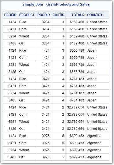
Simple Joins
/* FedSQL code for simple join */
proc fedsql;
   title 'Simple Join - GrainProducts and Sales';
   select * from grainproducts, sales;
quit;
/* FedSQL code for equijoin */
proc fedsql;
   title 'Equijoin - GrainProducts and Sales';
   select * from grainproducts, sales
      where grainproducts.prodid=sales.prodid;
quit; 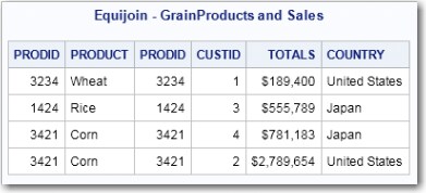
Cross Joins
Inner Joins

proc fedsql;
   title 'Inner Join - GrainProducts and Sales';
   select *
      from grainproducts inner join sales
         on grainproducts.prodid=sales.prodid;
quit;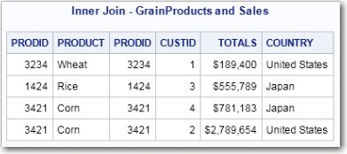
select *
   from grainproducts inner join sales
      on grainproducts.prodid=sales.prodid;
select *
from grainproducts inner join sales
using (prodid);This code produces the same output
as the previous code but uses the inner join construction. select *
from grainproducts, sales
where grainproducts.prodid=sales.prodid; Outer Joins
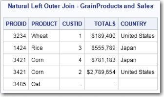
Left Outer Joins

title 'Left Outer Join - GrainProducts and Sales';
select *
   from grainproducts left outer join sales
      on grainproducts.prodid=sales.prodid;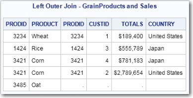
Right Outer Joins

title 'Right Outer Join - GrainProducts and Sales';
select *
   from grainproducts right outer join sales
      on grainproducts.prodid=sales.prodid;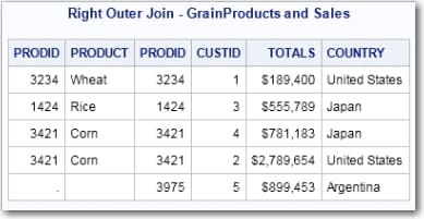
Full Outer Joins

title 'Full Outer Join - GrainProducts and Sales';
select *
   from grainproducts full outer join sales
      on grainproducts.prodid=sales.prodid;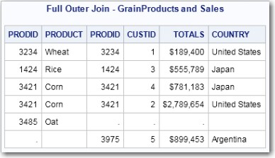
ON and USING Clauses
United
                           States
from the results table.title 'Inner Join - GrainProducts and Sales Outside US';
select *
from grainproducts inner join sales
on sales.country <> 'United States'
AND grainproducts.prodid=sales.prodid;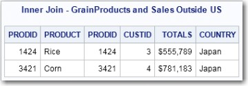
Natural Joins
WHERE Clause
Arguments
<search-condition>
specifies the conditions for the rows returned by the WHERE clause.
| See | <search-condition> |
Details
where max(inventory1)>10000;However, you can use this WHERE clause.
where max(inventory1, inventory2)>10000;
GROUP BY Clause
Arguments
column
specifies the name of a column or a column alias.
column-position-number
specifies a nonnegative integer that equates to a column position.
<sql-expression>
specifies a valid SQL expression.
| See | <sql-expression> |
Details
select x, sum(y)
   from table1
   group by x;
select sum(x), y
   from table1
   group by y;
HAVING Clause
Arguments
<search-condition>
specifies the conditions for the rows returned by the HAVING clause.
| See | <search-condition> |
Details
ORDER BY Clause
Syntax
[, ...order-by-expression [COLLATE collating-sequence-options]]
Arguments
order-by-expression
specifies a column on which to sort. The sort column can be one of the following.
column
specifies the name of a column or a column alias.
column-position-number
specifies a nonnegative integer that equates to a column position.
<sql-expression>
specifies any valid SQL expression.
| See | <sql-expression> |
ASC
orders the data in ascending order. This is the default order; if ASC or DESC are not specified, the data is ordered in ascending order.
DESC
orders the data in descending order.
COLLATE collating-sequence-options
specifies linguistic collation, which sorts characters according to rules of the specified language. The rules and default collating sequence options are based on the language specified in the current locale setting. The implementation is provided by the International Components for Unicode (ICU) library and produces results that are largely compatible with the Unicode Collation Algorithms (UCA).
DANISH | FINNISH | ITALIAN | NORWEGIAN | POLISH | SPANISH | SWEDISH
sorts characters according to the language specified.
LINGUISTIC [collating-rules]
collating-rules can be one of the following values:
ALTERNATE_HANDLING=SHIFTED
controls the handling of variable characters like spaces, punctuation, and symbols. When this option is not specified (using the default value NON_IGNORABLE), differences among these variable characters are of the same importance as differences among letters. If the ALTERNATE_HANDLING option is specified, these variable characters are of minor importance.
| Default | NON_IGNORABLE |
| Tip | The SHIFTED value is often used in combination with STRENGTH= set to Quaternary. In such a case, spaces, punctuation, and symbols are considered when comparing strings, but only if all other aspects of the strings (base letters, accents, and case) are identical. |
CASE_FIRST=
specify order of uppercase and lowercase letters. This argument is valid for only TERTIARY, QUATERNARY, or IDENTICAL levels. The following table provides the values and information for the CASE_FIRST argument:
COLLATION=
LOCALE= locale_name
specifies the locale name in the form of a POSIX name(for example, ja_JP). For more information, see SAS National Language Support (NLS): Reference Guide
NUMERIC_COLLATION=
STRENGTH=
| Restriction | Linguistic collation is not supported on platforms VMS on Itanium (VMI) or 64-bit Windows on Itanium (W64). |
| Tip | The collating-rules must be enclosed in parentheses. More than one collating rule can be specified. |
| See | ICU License - ICU 1.8.1 and later. |
| The section on Linguistic Collation in SAS National Language Support (NLS): Reference Guide. | |
| Refer to http://www.unicode.org for the Unicode Collation Algorithm (UCA) specification. |
Details
LIMIT Clause
OFFSET Clause
UNION Operator
Arguments
<query-specification> | <query-expression>
specifies one or more SELECT statements that produces a virtual table.
| See | SELECT Statement |
| Overview of Subqueries |
UNION
specifies that multiple result tables are combined and returned as a single result table.
ALL
specifies that all rows, including duplicates, are included in the result table. If not specified, all rows are returned.
DISTINCT
specifies that only unique rows can appear in the result table.
| See | DISTINCT Predicate |
Details
EXCEPT Operator
Arguments
<query-specification> | <query-expression>
specifies one or more SELECT statements that produces a virtual table.
| See | SELECT Statement |
| Overview of Subqueries |
EXCEPT
specifies that multiple result tables are combined and only those rows that are in the first result table and not in the second result table are included.
ALL
specifies that all rows, including duplicates, are included in the result table. If not specified, all rows are returned.
DISTINCT
specifies that only unique rows can appear in the result table.
| See | DISTINCT Predicate |
CORRESPONDING
specifies the columns to include in the query.
| Tip | If you do not specify the BY clause, the result table will include every column that appears in both of the tables. |
BY
specifies that only these columns be included in the result table.
column
specifies the name of the column.
| Restriction | Every column must be a valid column in both tables. |
Details
INTERSECT Operator
Arguments
<query-specification> | <query-expression>
specifies one or more SELECT statements that produces a virtual table.
| See | SELECT Statement |
| Overview of Subqueries |
INTERSECT
specifies that multiple result tables are combined and only those rows that are common to both result tables are included.
ALL
specifies that all rows, including duplicates, are included in the result table. If not specified, all rows are returned.
DISTINCT
specifies that only unique rows can appear in the result table.
| See | DISTINCT Predicate |
CORRESPONDING
specifies the columns to include in the query.
| Tip | If you do not specify the BY clause, the result table will include every column that appears in both of the tables. |
BY
specifies that only these columns to be included in the result table.
column
specifies the name of the column.
| Restriction | Every column must be a valid column in both tables. |
Details
<search-condition>
Syntax
[{AND | OR} [NOT] {<sql-expression> | (<search-condition>)}]}]
Arguments
NOT
AND
combines two conditions by finding observations that satisfy both conditions. This table outlines the outcomes when you compare TRUE and FALSE values using the AND operator.
OR
combines two conditions by finding observations that satisfy either condition or both. This table outlines the outcomes when you compare TRUE and FALSE values using the OR operator.
<sql-expression>
specifies any valid SQL expression.
| See | <sql-expression> |
Details
select * from test where x = cast (1.0e20 as real);
select cast (1.0e20 as real) from test;
select cast (col1 as real) from test;