The UCM Procedure
- Overview
-
Getting Started

-
SyntaxFunctional SummaryPROC UCM StatementAUTOREG StatementBLOCKSEASON StatementBY StatementCYCLE StatementDEPLAG StatementESTIMATE StatementFORECAST StatementID StatementIRREGULAR StatementLEVEL StatementMODEL StatementNLOPTIONS StatementOUTLIER StatementPERFORMANCE StatementRANDOMREG StatementSEASON StatementSLOPE StatementSPLINEREG StatementSPLINESEASON Statement
-
Details
-
Examples
- References
An Introduction to Unobserved Component Models
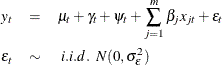
A UCM decomposes the response series into components such as trend, seasons, cycles, and the regression effects due to predictor series. The following model shows a possible scenario:
The terms  , and
, and  represent the trend, seasonal, and cyclical components, respectively. In fact the model can contain multiple seasons and
cycles, and the seasons can be of different types. For simplicity of discussion the preceding model contains only one of each
of these components. The regression term,
represent the trend, seasonal, and cyclical components, respectively. In fact the model can contain multiple seasons and
cycles, and the seasons can be of different types. For simplicity of discussion the preceding model contains only one of each
of these components. The regression term,  , includes contribution of regression variables with fixed regression coefficients. A model can also contain regression variables that have time varying regression coefficients or that have a nonlinear relationship with the dependent series (see Incorporating Predictors of Different Kinds). The disturbance term
  , also called the irregular component, is usually assumed to be Gaussian white noise. In some cases it is useful to model the irregular component as
a stationary ARMA process. See the section Modeling the Irregular Component for additional information.
, also called the irregular component, is usually assumed to be Gaussian white noise. In some cases it is useful to model the irregular component as
a stationary ARMA process. See the section Modeling the Irregular Component for additional information.
By controlling the presence or absence of various terms and by choosing the proper flavor of the included terms, the UCMs can generate a rich variety of time series patterns. A UCM can be applied to variables after transforming them by transforms such as log and difference.
The components , and model structurally different aspects of the time series. For example, the trend  models the natural tendency of the series in the absence of any other perturbing effects such as seasonality, cyclical components,
and the effects of exogenous variables, while the seasonal component
models the natural tendency of the series in the absence of any other perturbing effects such as seasonality, cyclical components,
and the effects of exogenous variables, while the seasonal component  models the correction to the level due to the seasonal effects. These components are assumed to be statistically independent
of each other and independent of the irregular component. All of the component models can be thought of as stochastic generalizations
of the relevant deterministic patterns in time. This way the deterministic cases emerge as special cases of the stochastic
models. The different models available for these unobserved components are discussed next.
models the correction to the level due to the seasonal effects. These components are assumed to be statistically independent
of each other and independent of the irregular component. All of the component models can be thought of as stochastic generalizations
of the relevant deterministic patterns in time. This way the deterministic cases emerge as special cases of the stochastic
models. The different models available for these unobserved components are discussed next.
Modeling the Trend
As mentioned earlier, the trend in a series can be loosely defined as the natural tendency of the series in the absence of
any other perturbing effects. The UCM procedure offers two ways to model the trend component . The first model, called the random walk (RW) model, implies that the trend remains roughly constant throughout the life
of the series without any persistent upward or downward drift. In the second model the trend is modeled as a locally linear
time trend (LLT). The RW model can be described as

Note that if  , then the model becomes
  . In the LLT model the trend is locally linear, consisting of both the level and slope. The LLT model is
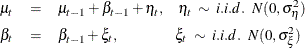
The disturbances  and
and  are assumed to be independent. There are some interesting special cases of this model obtained by setting one or both of
the disturbance variances
are assumed to be independent. There are some interesting special cases of this model obtained by setting one or both of
the disturbance variances  and
and  equal to zero. If is set equal to zero, then you get a linear trend model with fixed slope. If is set to zero, then the resulting model usually has a smoother trend. If both the variances are set to zero, then the resulting
model is the deterministic linear time trend:
equal to zero. If is set equal to zero, then you get a linear trend model with fixed slope. If is set to zero, then the resulting model usually has a smoother trend. If both the variances are set to zero, then the resulting
model is the deterministic linear time trend:  .
.
You can incorporate these trend patterns in your model by using the LEVEL and SLOPE statements.
Modeling a Cycle
A deterministic cycle with frequency  ,
,  , can be written as
![\[ \psi _ t = \alpha \cos ( \lambda t ) + \beta \sin ( \lambda t ) \]](images/etsug_ucm0132.png)
If the argument t is measured on a continuous scale, then is a periodic function with period  , amplitude
 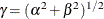 , and phase
  . Equivalently, the cycle can be written in terms of the amplitude and phase as
![\[ \psi _ t = \gamma \cos (\lambda t - \phi ) \]](images/etsug_ucm0136.png)
Note that when is measured only at the integer values, it is not exactly periodic, unless  for some integers j and k. The cycles in their pure form are not used very often in practice. However, they are very useful as building blocks for
more complex periodic patterns. It is well known that the periodic pattern of any complexity can be written as a sum of pure
cycles of different frequencies and amplitudes. In time series situations it is useful to generalize this simple cyclical
pattern to a stochastic cycle that has a fixed period but time-varying amplitude and phase. The stochastic cycle considered
here is motivated by the following recursive formula for computing :
for some integers j and k. The cycles in their pure form are not used very often in practice. However, they are very useful as building blocks for
more complex periodic patterns. It is well known that the periodic pattern of any complexity can be written as a sum of pure
cycles of different frequencies and amplitudes. In time series situations it is useful to generalize this simple cyclical
pattern to a stochastic cycle that has a fixed period but time-varying amplitude and phase. The stochastic cycle considered
here is motivated by the following recursive formula for computing :
![\[ \left[ \begin{array}{c} \psi _{t} \\ \psi ^{*}_{t} \end{array} \right] = \left[ \begin{array}{lr} \cos \lambda & \sin \lambda \\ - \sin \lambda & \cos \lambda \end{array} \right] \left[ \begin{array}{c} \psi _{t-1} \\ \psi ^{*}_{t-1} \end{array} \right] \]](images/etsug_ucm0138.png)
starting with  and
and  . Note that and
  satisfy the relation
![\[ \psi _{t}^{2} + \psi _{t}^{* 2} = \alpha ^2 + \beta ^2 \; \; \; \; \; \mr{for \; all} \; \; t \]](images/etsug_ucm0142.png)
A stochastic generalization of the cycle can be obtained by adding random noise to this recursion and by introducing a damping factor,  , for additional modeling flexibility. This model can be described as follows
![\[ \left[ \begin{array}{c} \psi _{t} \\ \psi ^{*}_{t} \end{array} \right] = \rho \left[ \begin{array}{lr} \cos \lambda & \sin \lambda \\ - \sin \lambda & \cos \lambda \end{array} \right] \left[ \begin{array}{c} \psi _{t-1} \\ \psi ^{*}_{t-1} \end{array} \right] + \left[ \begin{array}{c} \nu _{t} \\ \nu ^{*}_{t} \end{array} \right] \]](images/etsug_ucm0029.png)
where  , and the disturbances
  and
and  are independent
  variables. The resulting stochastic cycle has a fixed period but time-varying amplitude and phase. The stationarity properties
of the random sequence depend on the damping factor . If
variables. The resulting stochastic cycle has a fixed period but time-varying amplitude and phase. The stationarity properties
of the random sequence depend on the damping factor . If  , has a stationary distribution with mean zero and variance
  . If
. If  , is nonstationary.
You can incorporate a cycle in a UCM by specifying a CYCLE statement. You can include multiple cycles in the model by using separate CYCLE statements for each included cycle.
As mentioned before, the cycles are very useful as building blocks for constructing more complex periodic patterns. Periodic patterns of almost any complexity can be created by superimposing cycles of different periods and amplitudes. In particular, the seasonal patterns, general periodic patterns with integer periods, can be constructed as sums of cycles. This important topic of modeling the seasonal components is considered next.
Modeling Seasons
The seasonal fluctuations are a common source of variation in time series data. These fluctuations arise because of the regular
changes in seasons or some other periodic events. The seasonal effects are regarded as corrections to the general trend of
the series due to the seasonal variations, and these effects sum to zero when summed over the full season cycle. Therefore
the seasonal component  is modeled as a stochastic periodic pattern of an integer period s such that the sum
  is always zero in the mean. The period s is called the season length. Two different models for the seasonal component are considered here. The first model is called
the dummy variable form of the seasonal component. It is described by the equation
is always zero in the mean. The period s is called the season length. Two different models for the seasonal component are considered here. The first model is called
the dummy variable form of the seasonal component. It is described by the equation
![\[ \sum _{i=0}^{s-1} \gamma _{t-i} = \omega _ t , \; \; \; \; \; \; \; \; \; \; \; \; \omega _ t \; \sim \; i.i.d. \; \; N( 0, \sigma _{\omega }^{2} ) \]](images/etsug_ucm0095.png)
The other model is called the trigonometric form of the seasonal component. In this case is modeled as a sum of cycles of different frequencies. This model is given as follows
![\[ \gamma _ t = \sum _{j = 1}^{[s/2]} \gamma _{j,t} \]](images/etsug_ucm0096.png)
where ![$[s/2]$](images/etsug_ucm0097.png) equals
equals  if s is even and
  if it is odd. The cycles
  have frequencies
  and are specified by the matrix equation
![\[ \left[ \begin{array}{c} \gamma _{j,t} \\ \gamma ^{*}_{j,t} \end{array} \right] = \left[ \begin{array}{lr} \cos \lambda _ j & \sin \lambda _ j \\ - \sin \lambda _ j & \cos \lambda _ j \end{array} \right] \left[ \begin{array}{c} \gamma _{j,t-1} \\ \gamma ^{*}_{j,t-1} \end{array} \right] + \left[ \begin{array}{c} \omega _{j,t} \\ \omega ^{*}_{j,t} \end{array} \right] \]](images/etsug_ucm0102.png)
where the disturbances  and
and  are assumed to be independent and, for fixed j, and
  . If s is even, then the equation for
  is not needed and
  is given by
![\[ \gamma _{s/2,t} = - \gamma _{s/2,t-1} + \omega _{s/2,t} \]](images/etsug_ucm0108.png)
The cycles are called harmonics. If the seasonal component is deterministic, the decomposition of the seasonal effects into these harmonics is identical
to its Fourier decomposition. In this case the sum of squares of the seasonal factors equals the sum of squares of the amplitudes
of these harmonics. In many practical situations, the contribution of the high-frequency harmonics is negligible and can be
ignored, giving rise to a simpler description of the seasonal. In the case of stochastic seasonals, the situation might not
be so transparent; however, similar considerations still apply. Note that if the disturbance variance  , then both the dummy and the trigonometric forms of seasonal components reduce to constant seasonal effects. That is, the
seasonal component reduces to a deterministic function that is completely determined by its first
, then both the dummy and the trigonometric forms of seasonal components reduce to constant seasonal effects. That is, the
seasonal component reduces to a deterministic function that is completely determined by its first  values.
In the UCM procedure you can specify a seasonal component in a variety of ways, the SEASON
statement being the simplest of these. The dummy and the trigonometric seasonal components discussed so far can be considered
as saturated seasonal components that put no restrictions on the seasonal values. In some cases a more parsimonious representation of the seasonal might be more appropriate. This is particularly
useful for seasonal components with large season lengths. In the UCM procedure you can obtain parsimonious representations
of the seasonal components by one of the following ways:
-
Use a subset trigonometric seasonal component obtained by deleting a few of the
harmonics used in its sum. For example, a slightly smoother seasonal component of length 12, corresponding to the monthly
seasonality, can be obtained by deleting the highest-frequency harmonic of period 2. That is, such a seasonal component will
be a sum of five stochastic cycles that have periods 12, 6, 4, 3, and 2.4. You can specify such subset seasonal components
by using the KEEPH=
or DROPH=
option in the SEASON
statement.
-
Approximate the seasonal pattern by a suitable spline approximation. You can do this by using the SPLINESEASON statement.
-
A block-seasonal pattern is a seasonal pattern where the pattern is divided into a few blocks of equal length such that the season values within a block are the same—for example, a monthly seasonal pattern that has only four different values, one for each quarter. In some situations a long seasonal pattern can be approximated by the sum of block season and a simple season, the length of the simple season being equal to the block length of the block season. You can obtain such approximation by using a combination of BLOCKSEASON and SEASON statements.
-
Consider a seasonal component of a large season length as a sum of two or more seasonal components that are each of much smaller season lengths. This can be done by specifying more than one SEASON statements.
Note that the preceding techniques of obtaining parsimonious seasonal components can also enable you to specify seasonal components that are more general than the simple saturated seasonal components. For example, you can specify a saturated trigonometric seasonal component that has some of its harmonics evolving according to one disturbance variance parameter while the others evolve with another disturbance variance parameter.
Modeling an Autoregression
An autoregression of order one can be thought of as a special case of a cycle when the frequency is either 0 or  . Modeling this special case separately helps interpretation and parameter estimation. The autoregression component
  is modeled as follows
![\[ r_ t = \rho r_{t-1} + \nu _{t} , \; \; \; \; \nu _ t \; \sim \; i.i.d. \; \; N( 0, \sigma _{\nu }^{2} ) \]](images/etsug_ucm0017.png)
where  . An autoregression can also provide an alternative to the IRREGULAR
component when the model errors show some autocorrelation. You can incorporate an autoregression in your model by using the
AUTOREG
statement.
. An autoregression can also provide an alternative to the IRREGULAR
component when the model errors show some autocorrelation. You can incorporate an autoregression in your model by using the
AUTOREG
statement.
Modeling Regression Effects
A predictor variable can affect the response variable in a variety of ways. The UCM procedure enables you to model several different types of predictor-response relationships:
-
The predictor-response relationship is linear, and the regression coefficient does not change with time. This is the simplest kind of relationship and such predictors are specified in the MODEL statement.
-
The predictor-response relationship is linear, but the regression coefficient does change with time. Such predictors are specified in the RANDOMREG statement. Here the regression coefficient is assumed to evolve as a random walk.
-
The predictor-response relationship is nonlinear and the relationship can change with time. This type of relationship can be approximated by an appropriate time-varying spline. Such predictors are specified in the SPLINEREG statement.
A response variable can depend on its own past values—that is, lagged dependent values. Such a relationship can be specified in the DEPLAG statement.
Modeling the Irregular Component
The components—such as trend, seasonal and regression effects, and nonstationary cycles—are used to capture the structural
dynamics of a response series. In contrast, the stationary cycles and the autoregression are used to capture the transient
aspects of the response series that are important for its short-range prediction but have little impact on its long-term forecasts.
The irregular component represents the residual variation remaining in the response series that is modeled using an appropriate
selection of structural and transient effects. In most cases, the irregular component can be assumed to be simply Gaussian
white noise. In some other cases, however, the residual variation can be more complicated. In such situations, it might be
necessary to model the irregular component as a stationary ARMA process. Moreover, you can use the ARMA irregular component
together with the dependent lag specification (see the DEPLAG
statement) to specify an ARIMA(p,d,q) (P,D,Q)
 model for the response series. See the IRREGULAR
statement for the explanation of the ARIMA notation. See Example 41.8 for an example of modeling a series by using an ARIMA(0,1,1)(0,1,1)
model for the response series. See the IRREGULAR
statement for the explanation of the ARIMA notation. See Example 41.8 for an example of modeling a series by using an ARIMA(0,1,1)(0,1,1) model.
The Model Parameters
The parameter vector in a UCM consists of the variances of the disturbance terms of the unobserved components, the damping coefficients and frequencies in the cycles, the damping coefficient in the autoregression, and the regression coefficients in the regression terms. These parameters are estimated by maximizing the likelihood. It is possible to restrict the values of the model parameters to user-specified values.
Model Specification
A UCM is specified by describing the components in the model. For example, consider the model
![\[ {y}_ t = \mu _ t + \gamma _ t + \epsilon _ t \]](images/etsug_ucm0006.png)
consisting of the irregular, level, slope, and seasonal components. This model is called the basic structural model (BSM) by Harvey (1989). The syntax for a BSM with monthly seasonality of trigonometric type is as follows:
   model y;
   irregular;
   level;
   slope;
   season length=12 type=trig;
Similarly the following syntax specifies a BSM with a response variable y, a regressor x, and dummy-type monthly seasonality:
   model y = x;
   irregular;
   level;
   slope variance=0 noest;
   season length=12 type=dummy;
Moreover, the disturbance variance of the slope component is restricted to zero, giving rise to a local linear trend with fixed slope.
A model can contain multiple cycle and seasonal components. In such cases the model syntax contains a separate statement for each of these multiple cycle or seasonal components; for example, the syntax for a model containing irregular and level components along with two cycle components could be as follows:
   model y = x;
   irregular;
   level;
   cycle;
   cycle;