The TIMEDATA Procedure

This example demonstrates the use of the AUXDATA= option in PROC TIMEDATA. The data set Sashelp.Gulfoil contains oil and gas production data from the Gulf of Mexico. The variables RegionName and ProtractionName can be used to define a time series hierarchy of interest. Suppose you want to generate two new series that contain the protraction’s share of oil and gas production for its associated region at each time index.

You first use PROC TIMESERIES to perform temporal aggregation (accumulation) of the time series for the RegionName level.

proc timeseries data=sashelp.gulfoil
                out=byregion(rename=(oil=roil gas=rgas));
   by regionname;
   id date interval=month accumulate=total notsorted;
   var oil gas;
run;

You can then use PROC TIMEDATA with the AUXDATA= option to compute the share of oil and gas production contributed by each protraction within its associated region. PROC TIMEDATA reads a monthly time series for each (RegionName, ProtractionName) group for the variables Oil and Gas from Sashelp.Gulfoil. Two new series are produced in the variables Oilshare and Gasshare that respectively contain the protraction’s share of the oil and gas production at the region level of the hierarchy (given by variables Roil and Rgas). Those share variables are specified in the OUTARRAY statement for inclusion in the OUTARRAY= data set (Work.Shares). This example relies on the capability of the AUXDATA= feature to perform partial BY group matching. The time series that are acquired for the variables Roil and Rgas are the result of matching on the RegionName BY variable from the data set Work.Byregion with the RegionName variable from the BY groups that are acquired from the Sashelp.Gulfoil data set.

proc timedata data=sashelp.gulfoil
              auxdata=byregion
              out=_null_
              outarray=shares;
   by regionname protractionname;
   outarray oilshare gasshare;
   var oil gas roil rgas;
   id date interval=month accumulate=total;
   do i=1 to _length_;
      oilshare[i] = oil[i] / roil[i];
      gasshare[i] = gas[i] / rgas[i];
   end;
run;

The following code demonstrates that the computed shares sum to 1 for each time index in the resulting Oilshare and Gasshare series. PROC TIMESERIES is used to accumulate the shares for these respective variables from the data set Work.Shares and the accumulated share series at the RegionName level are stored to the data set Work.Rshares with variable names Oilsum and Gassum, respectively. The summary from PROC MEANS for the distinct values of RegionName shows that per-time totals for both share series sums to 1.

proc timeseries data=shares
                out=rshares(rename=(oilshare=oilsum gasshare=gassum));
   by regionname;
   id date interval=month accumulate=total notsorted;
   var oilshare gasshare;
run;
proc means data=rshares;
   by regionname;
   var oilsum gassum;
run;

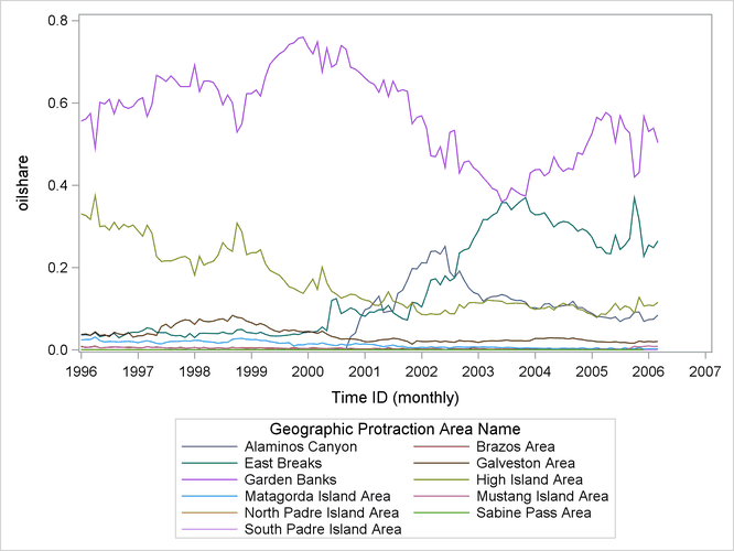
You might also want to plot the share series. The following code produces a graph that overlays the protraction level share series for oil production for the Western region.

proc sgplot data=shares(where=(RegionName='Western'));
   series x=Date y=OilShare/group=ProtractionName;
run;

Output 37.3.2: Protraction Share of Oil Production for Western Region