Specifying Forecasting Models

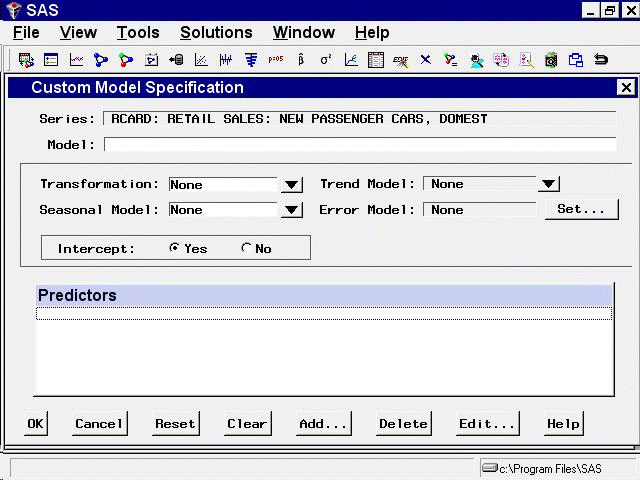
To fit a custom time series model not already provided in the Models to Fit window, select the Custom Model item from the pop-up menu, toolbar, or Edit menu. This opens the Custom Model Specification window, as shown in Figure 56.19.

You can specify the same time series models with the Custom Model Specification window and the ARIMA Model Specification window, but the windows are structured differently, and you might find one more convenient than the other.

At the top of the Custom Model Specification window is the name and label of the series and the label of the model you are specifying. The model label is filled in with an automatically generated label as you specify options. You can type over the automatic label with your own label for the model. To restore the automatic label, enter a blank label.

The middle part of the Custom Model Specification window consists of four fields: Transformation, Trend Model, Seasonal Model, and Error Model. These fields allow you to specify the model in four parts. Each part specifies how a different aspect of the pattern of the time series is modeled and predicted.

The Predictors list at the bottom of the Custom Model Specification window allows you to include different kinds of predictor variables in the forecasting model. The Predictors feature for the Custom Model Specification window is like the Predictors feature for the ARIMA Model Specification window, except that time trend predictors are provided through the Trend Model field and seasonal dummy variable predictors are provided through the Seasonal Model field.

To illustrate how to use the Custom Model Specification window, the following example specifies the same model you fit by using the ARIMA Model Specification window.

First, specify the data transformation to use. Select "Log" using the Transformation combo box.

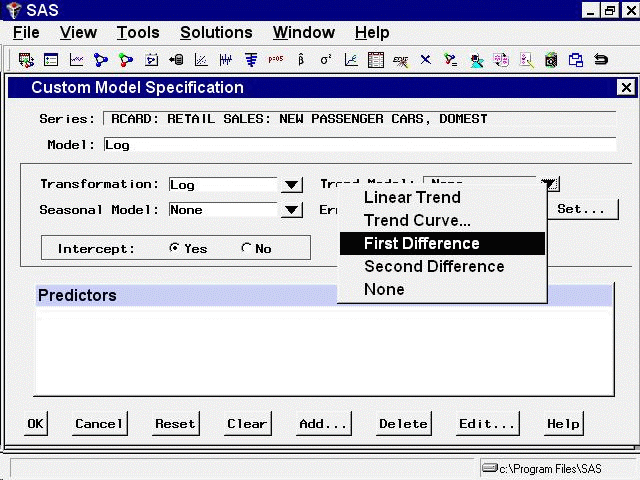
Second, specify how to model the trend in the series. Select First Difference in the Trend Model combo box, as shown in Figure 56.20.

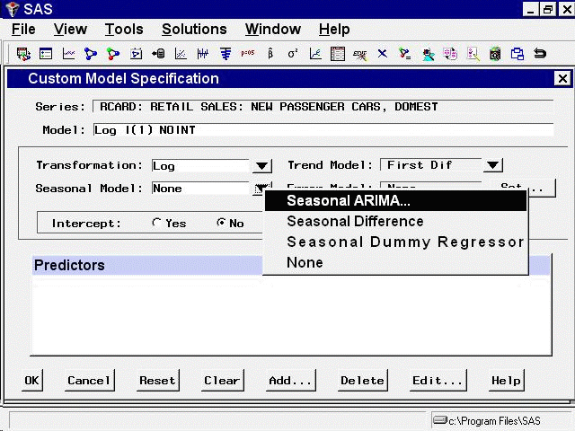
Next, specify how to model the seasonal pattern in the series. Select "Seasonal ARIMA" in the Seasonal Model combo box, as shown in Figure 56.21.

This opens the Seasonal ARIMA Model Options window, as shown in Figure 56.22.

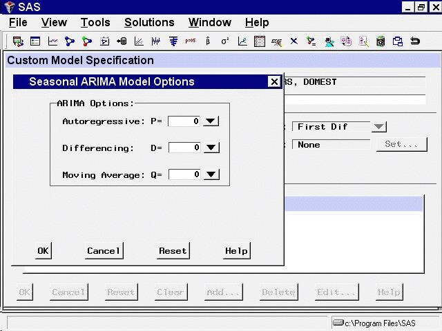
Specify a first-order seasonal moving-average term by typing 1 or by selecting "1" from the Moving Average: Q= combo box pop-up menu, and then select the OK button.

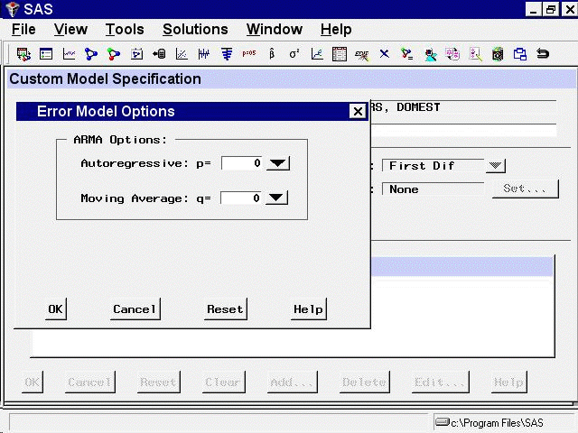
Finally, specify how to model the autocorrelation pattern in the model prediction errors. Select the Set button to the right of the Error Model field. This opens the Error Model Options window, as shown in Figure 56.23. This window allows you to specify an ARMA error process. Set the Moving Average order q to 2, and then select the OK button.

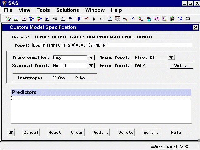
The Custom Model Specification window should now appear as shown in Figure 56.24. The model label at the top of the Custom Model Specification window should now read Log ARIMA(0,1,2)(0,0,1)s NOINT, just as it did when you used the ARIMA Model Specification window.

Now that you have seen how the Custom Model Specification window works, select "Cancel" to exit the window without fitting the model. This should return you to the Develop Models window.