Specifying Forecasting Models

To fit a factored ARIMA model, select the Factored ARIMA model item from the pop-up menu, toolbar, or Edit menu. This brings up the Factored ARIMA Model Specification window, shown in Figure 56.16.

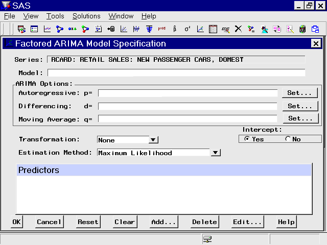
The Factored ARIMA Model Specification window is similar to the ARIMA Model Specification window and has the same features, but it uses a more general specification of the autoregressive (p), differencing (d), and moving-average (q) terms. To specify these terms, select the corresponding Set button, as shown in Figure 56.16. For example, to specify autoregressive terms, select the first Set button. This opens the AR Polynomial Specification Window, shown in Figure 56.17.

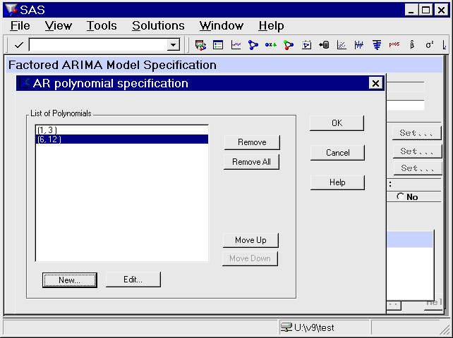
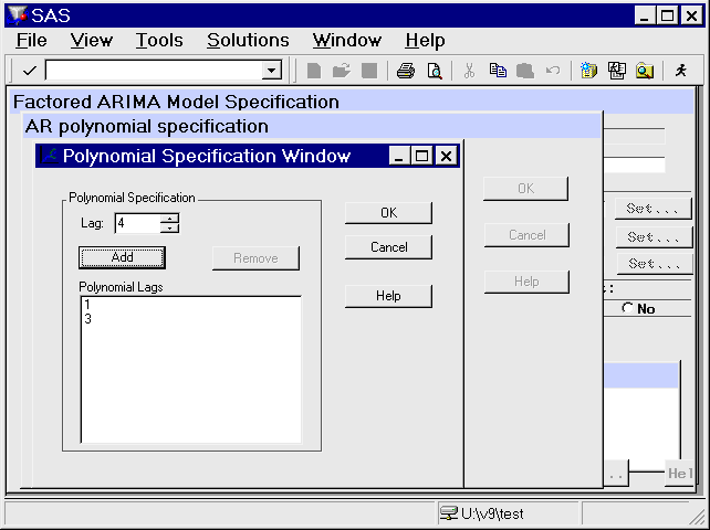
To add AR polynomial terms, select the New button. This opens the Polynomial Specification Window, shown in Figure 56.18. Specify the first lag you want to include by using the Lag spin box, then select the Add button. Repeat this process, adding each lag you want to include in the current list. All lags must be specified. For example, if you add only lag 3, the model contains only lag 3, not 1 through 3.

As an example, add lags 1 and 3, then select the OK button. The AR Polynomial Specification Window now shows (1,3) in the list of polynomials. Now select "New" again. Add lags 6 and 12 and select "OK". Now the AR Polynomial Specification Window shows (1,3) and (6,12) as shown in Figure 56.17. Select "OK" to close this window. The Factored ARIMA Model Specification Window now shows the factored model p=(1,3)(6,12). Use the same technique to specify the q terms, or moving-average part of the model. There is no limit to the number of lags or the number of factors you can include in the model.

To specify differencing lags, select the middle Set button to open the Differencing Specification window. Specify lags using the spin box and add them to the list with the Add button. When you select "OK" to close the window, the differencing lags appear after d= in the Factored ARIMA Specification Window, within a single pair of parentheses.

You can use the Factored ARIMA Model Specification Window to specify any model that you can specify with the ARIMA Model and Custom Model windows, but the notation is more similar to that of the ARIMA procedure (see Chapter 8: The ARIMA Procedure). Consider as an example the classic Airline model fit to the International Airline Travel series, SASHELP.AIR. This is a factored model with one moving-average term at lag one and one moving-average term at the seasonal lag, with first-order differencing at the simple and seasonal lags. Using the ARIMA Model Specification Window, you specify the value 1 for the q and d terms and also for the Q and D terms, which represent the seasonal lags. For monthly data, the seasonal lags represent lag 12, since a yearly seasonal cycle is assumed.

By contrast, the Factored ARIMA Model Specification Window makes no assumptions about seasonal cycles. The Airline model is written as IMA d=(1,12) q=(1)(12) NOINT. To specify the differencing terms, add the values 1 and 12 in the Differencing Specification Window and select OK. Then select "New" in the MA Polynomial Specification Window, add the value 1, and select OK. To add the factored term, select "New" again, add the value 12, and select OK. Remember to select "No" in the Intercept radio box, since it is not selected by default. Select OK to close the Factored ARIMA Model Specification Window and fit the model.

You can show that the results are the same as they are when you specify the model by using the ARIMA Model Specification Window and when you select Airline Model from the default model list. If you are familiar with the ARIMA Procedure (Chapter 8: The ARIMA Procedure), you might want to turn on the Show Source Statements option before fitting the model, then examine the procedure source statements in the log window after fitting the model.

The strength of the Factored ARIMA Specification approach lies in its ability to construct unusual ARIMA models, such as:

Models with high order lags take longer to fit and often fail to converge. To save time, select the Conditional Least Squares or Unconditional Least Squares estimation method (see Figure 56.16). Once you have narrowed down the list of candidate models, change to the Maximum Likelihood estimation method.