The SSM Procedure
-
Overview

- Getting Started
-
Syntax
-
DetailsState Space Model and NotationTypes of Sequence DataOverview of Model Specification SyntaxFiltering, Smoothing, Likelihood, and Structural Break DetectionEstimation of User-Specified Linear Combination of State ElementsContrasting PROC SSM with Other SAS Procedures Predefined Trend ModelsPredefined Structural ModelsModels with Dependent LagsCovariance ParameterizationMissing ValuesComputational IssuesDisplayed OutputODS Table NamesODS Graph NamesOUT= Data Set
-
ExamplesBivariate Basic Structural Model Panel Data: Random-Effects and Autoregressive ModelsBackcasting, Forecasting, and InterpolationLongitudinal Data: Smoothing of Repeated MeasuresA User-Defined Trend ModelModel with Multiple ARIMA ComponentsDynamic Factor ModelingDiagnostic Plots and Structural Break AnalysisLongitudinal Data: Variable Bandwidth SmoothingA Transfer Function Model for the Gas Furnace DataPanel Data: Dynamic Panel Model for the Cigar DataMultivariate Modeling: Long-Term Temperature TrendsBivariate Model: Sales of Mink and Muskrat FursFactor Model: Now-Casting the US EconomyLongitudinal Data: Lung Function Analysis
- References
Trend Models for Irregular Data
A good reference for these models is De Jong and Mazzi (2001). Throughout this section  denotes the difference between the successive time points. The system matrices
  and
and  that govern these models depend on
  . However, whenever the notation is unambiguous, the subscript t is omitted.
Polynomial Spline Trend
This model is a general-purpose tool for extracting a smooth trend from the noisy data. The order of the spline governs the order of the local polynomial that defines the spline. The order-1 spline corresponds to Brownian motion (continuous-time random walk), the order-2 spline corresponds to integrated Brownian motion (continuous-time integrated random walk), and the order-3 spline provides a locally quadratic trend; the default order is 1. The dimension of the state underlying this component is the same as the order of the spline. The system matrices for the orders up to 3 are described as follows (in all the cases the initial condition is fully diffuse):
-
order-1 spline:
 ,
,  , and
, and 
-
order-2 spline:
 ,
,  , and
, and 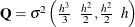
-
order-3 spline:
 ,
,  , and
, and
![\[ \mb{Q}[i, j] = \sigma ^{2}* \frac{h^{6-i-j+1}}{(6-i-j+1)(3-i)! (3-j)! } \; \; 1 \leq i, j \leq 3 \]](images/etsug_ssm0363.png)
The system matrices for higher orders are similarly defined (for more information, see De Jong and Mazzi (2001)).
Note that, in addition to providing an estimate of the trend, this methodology can provide estimates of the higher-order derivatives
of the trend. If  denotes the k-dimensional subsection that is associated with a polynomial spline of order k, then its
  th element (
 ),
), ![$\pmb {\alpha }[j]$](images/etsug_ssm0366.png) , corresponds to the derivative of order
, corresponds to the derivative of order  of this polynomial spline. For an example of the estimation of the first derivative of a trend component, see Example 34.12. For additional information about using these types of trend patterns in data analysis, see Eubank, Huang, and Wang (2003); Kohn, Ansley, and Tharm (1991); Selukar (2015).
Decay and Growth Trends
There are two choices for the decay trend: DECAY and DECAY(OU). Similarly, there are two choices for the growth trend: GROWTH and GROWTH(OU). The "OU" stands for the Ornstein-Uhlenbeck form of these models. The decay trend is a sum of two correlated components: one component is a random walk, and the other component is a stationary autoregression. In its Ornstein-Uhlenbeck form, the random walk component is replaced by a constant. The growth trend (and its Ornstein-Uhlenbeck variant) has the same form as the decay trend except that the autoregression is nonstationary (in fact, it is explosive). For growth trend models, floating-point errors can result for even moderately long forecast horizons because of the explosive growth in the trend values.
The system matrices for the decay and the growth types in their respective cases are identical, except for the sign of the
rate parameter  :
:  for the decay type, and
  for the growth type. In addition, the initial conditions for the growth models are fully diffuse; they are only partially
diffuse for the decay models. The underlying state vector for all these models is two-dimensional.
for the growth type. In addition, the initial conditions for the growth models are fully diffuse; they are only partially
diffuse for the decay models. The underlying state vector for all these models is two-dimensional.
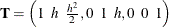
The system matrices for the DECAY type are:
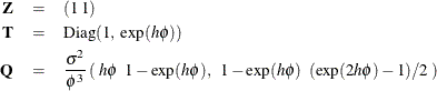
The initial condition is partially diffuse with 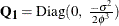 . The system matrices for the GROWTH type are the same (with ), except that the initial condition is fully diffuse; so
  .
.
For the DECAY(OU) type,  and
and  are the same as DECAY, whereas
![\[ \mb{Q}= \mr{Diag} \left(\; 0, \; \sigma ^{2} \frac{(\exp (2 h \phi ) - 1)}{2\phi } \; \right) \; \; \mr{and} \; \; \mb{Q_{1}}= \mr{Diag} (0, \; \frac{- \sigma ^{2}}{2 \phi } ) \]](images/etsug_ssm0373.png)
The system matrices for the GROWTH(OU) type are the same (with ), except that the initial condition is fully diffuse; so .