The SSM Procedure
-
Overview

- Getting Started
-
Syntax
-
DetailsState Space Model and NotationTypes of Sequence DataOverview of Model Specification SyntaxFiltering, Smoothing, Likelihood, and Structural Break DetectionEstimation of User-Specified Linear Combination of State ElementsContrasting PROC SSM with Other SAS Procedures Predefined Trend ModelsPredefined Structural ModelsModels with Dependent LagsCovariance ParameterizationMissing ValuesComputational IssuesDisplayed OutputODS Table NamesODS Graph NamesOUT= Data Set
-
ExamplesBivariate Basic Structural Model Panel Data: Random-Effects and Autoregressive ModelsBackcasting, Forecasting, and InterpolationLongitudinal Data: Smoothing of Repeated MeasuresA User-Defined Trend ModelModel with Multiple ARIMA ComponentsDynamic Factor ModelingDiagnostic Plots and Structural Break AnalysisLongitudinal Data: Variable Bandwidth SmoothingA Transfer Function Model for the Gas Furnace DataPanel Data: Dynamic Panel Model for the Cigar DataMultivariate Modeling: Long-Term Temperature TrendsBivariate Model: Sales of Mink and Muskrat FursFactor Model: Now-Casting the US EconomyLongitudinal Data: Lung Function Analysis
- References
Filtering Pass
The filtering pass sequentially computes the quantities shown in Table 34.5 for  and
and 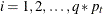 .
.
Table 34.5: KFS: Filtering Phase
|
Quantity |
Description |
|---|---|
|
|
One-step-ahead prediction of the response values |
|
|
One-step-ahead prediction residuals |
|
|
Variance of the one-step-ahead prediction |
|
|
One-step-ahead prediction of the state vector |
|
|
Covariance of |
|
|
|
|
|
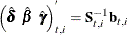
|
|
|
Estimates of |
|
|
Covariance of |


Here the notation  denotes the conditional expectation of
  given the history up to the index
  :
:  . Similarly
  denotes the corresponding conditional variance. The quantity
  is set to missing whenever
  is missing. Note that
  are one-step-ahead forecasts only when the model has only one response variable and the data are a time series; in all other cases it is more
appropriate to call them one-measurement-ahead forecasts (since the next measurement might be at the same time point). Despite this, are called one-step-ahead predictions (and
are one-step-ahead forecasts only when the model has only one response variable and the data are a time series; in all other cases it is more
appropriate to call them one-measurement-ahead forecasts (since the next measurement might be at the same time point). Despite this, are called one-step-ahead predictions (and  are called one-step-ahead residuals) throughout this document. In the diffuse case, the conditional expectations must be
appropriately interpreted. The vector
are called one-step-ahead residuals) throughout this document. In the diffuse case, the conditional expectations must be
appropriately interpreted. The vector  and the matrix
  contain some accumulated quantities that are needed for the estimation of
  ,
,  , and
, and  . Of course, when
  (the nondiffuse case), these quantities are not needed. In the diffuse case, because the matrix is sequentially accumulated (starting at
  ), it might not be invertible until some
  . The filtering process is called initialized after . In some situations, this initialization might not happen even after the entire sample is processed—that is, the filtering
process remains uninitialized. This can happen if the regression variables are collinear or if the data are not sufficient to estimate the initial condition
for some other reason.
. The filtering process is called initialized after . In some situations, this initialization might not happen even after the entire sample is processed—that is, the filtering
process remains uninitialized. This can happen if the regression variables are collinear or if the data are not sufficient to estimate the initial condition
for some other reason.
The filtering process is used for a variety of purposes. One important use of filtering is to compute the likelihood of the
data. In the model-fitting phase, the unknown model parameters  are estimated by maximum likelihood. This requires repeated evaluation of the likelihood at different trial values of . After is estimated, it is treated as a known vector. The filtering process is used again with the fitted model in the forecasting
phase, when the one-step-ahead forecasts and residuals based on the fitted model are provided. In addition, this filtering
output is needed by the smoothing phase to produce the full-sample component estimates and for the structural break analysis.
are estimated by maximum likelihood. This requires repeated evaluation of the likelihood at different trial values of . After is estimated, it is treated as a known vector. The filtering process is used again with the fitted model in the forecasting
phase, when the one-step-ahead forecasts and residuals based on the fitted model are provided. In addition, this filtering
output is needed by the smoothing phase to produce the full-sample component estimates and for the structural break analysis.