The SIMILARITY Procedure
- Overview
- Getting Started
-
Syntax

-
DetailsAccumulationMissing Value InterpretationZero Value InterpretationTime Series TransformationTime Series DifferencingTime Series Missing Value TrimmingTime Series Descriptive StatisticsInput and Target SequencesSliding SequencesTime WarpingSequence NormalizationSequence ScalingSimilarity MeasuresUser-Defined Functions and SubroutinesOutput Data SetsOUT= Data SetOUTMEASURE= Data SetOUTPATH= Data SetOUTSEQUENCE= Data SetOUTSUM= Data Set_STATUS_ Variable ValuesPrinted OutputODS Table NamesODS Graphics
-
Examples
- References
Example 31.2 Similarity Analysis
This simple example illustrates how to use similarity analysis to compare two time sequences. The following statements create an example data set that contains two time sequences of differing lengths:
data test;
input i y x;
datalines;
1   2  3
2   4  5
3   6  3
4   7  3
5   3  3
6   8  6
7   9  3
8   3  8
9  10  .
10 11  .
;
run;
The following statements perform similarity analysis on the example data set:
proc similarity data=test out=_null_
   print=all plot=all;
   input x;
   target y / measure=absdev;
run;
The DATA=TEST option specifies that the input data set WORK.TEST is to be used in the analysis. The OUT=_NULL_ option specifies that no output time series data set is to be created. The
PRINT=ALL and PLOTS=ALL options specify that all ODS tables and graphs are to be produced. The INPUT statement specifies that
the input variable is X. The TARGET statement specifies that the target variable is Y and that the similarity measure is computed using absolute deviation (MEASURE=ABSDEV).
Output 31.2.1: Description Statistics of the Input Variable, x
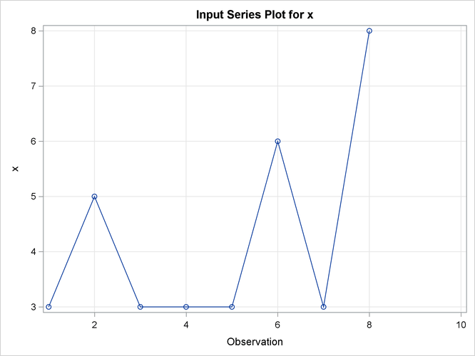
Output 31.2.2: Plot of Input Variable, x
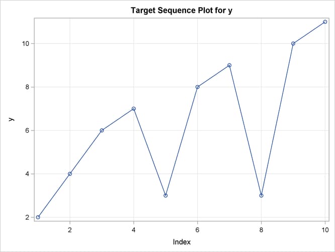
Output 31.2.3: Target Sequence Plot
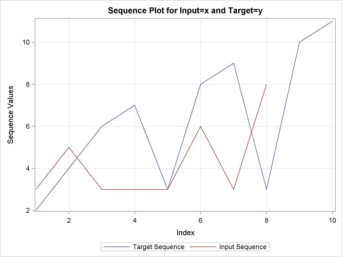
Output 31.2.4: Sequence Plot
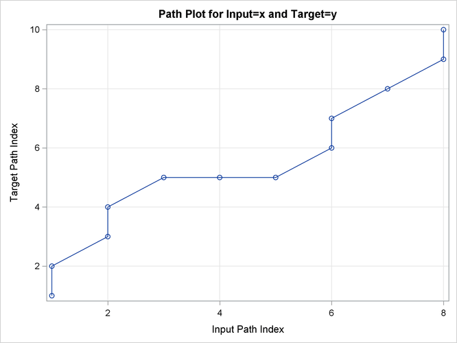
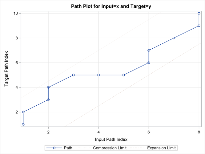
Output 31.2.5: Path Plot
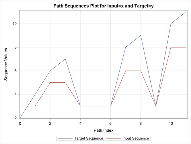
Output 31.2.6: Path Sequences Plot
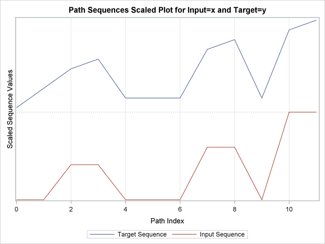
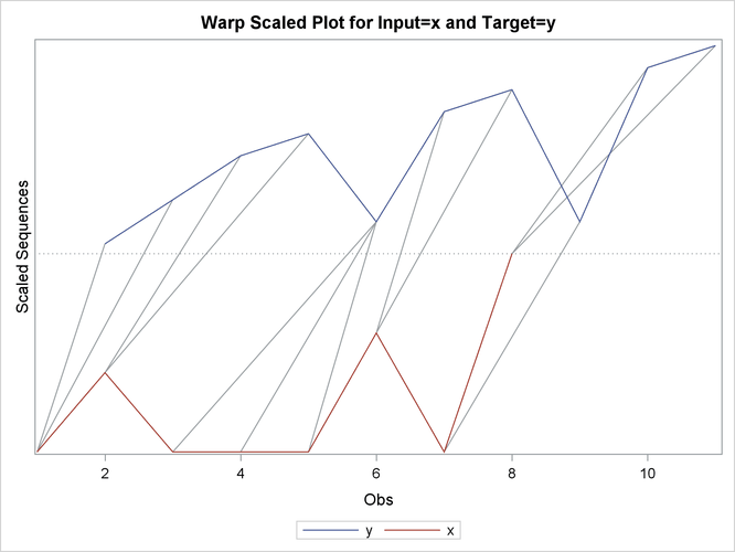
Output 31.2.7: Path Sequences Scaled Plot
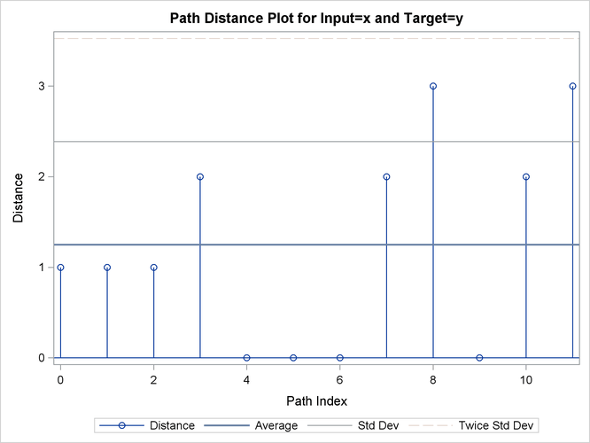
Output 31.2.8: Path Distance Plot
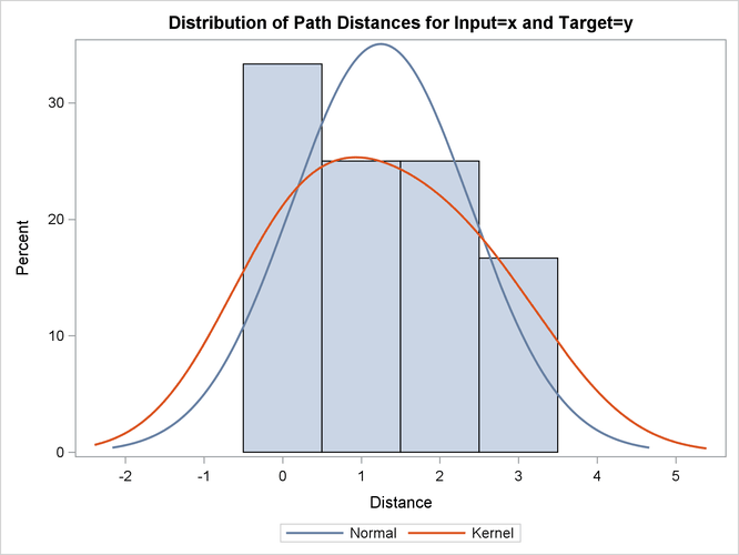
Output 31.2.9: Path Distance Histogram
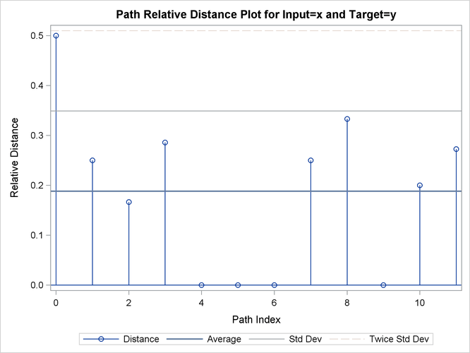
Output 31.2.10: Path Relative Distance Plot
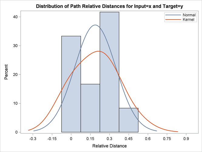
Output 31.2.11: Path Relative Distance Histogram
Output 31.2.12: Path Limits
Output 31.2.13: Path Statistics
| Path Statistics | ||||||||
|---|---|---|---|---|---|---|---|---|
| Path | Number | Path Percent | Input Percent | Target Percent | Maximum | Path Maximum Percent |
Input Maximum Percent |
Target Maximum Percent |
| Missing Map | 0 | 0.000% | 0.000% | 0.000% | 0 | 0.000% | 0.000% | 0.000% |
| Direct Maps | 6 | 50.00% | 75.00% | 60.00% | 2 | 16.67% | 25.00% | 20.00% |
| Compression | 4 | 33.33% | 50.00% | 40.00% | 1 | 8.333% | 12.50% | 10.00% |
| Expansion | 2 | 16.67% | 25.00% | 20.00% | 2 | 16.67% | 25.00% | 20.00% |
| Warps | 6 | 50.00% | 75.00% | 60.00% | 2 | 16.67% | 25.00% | 20.00% |
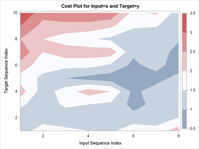
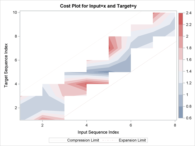
Output 31.2.14: Cost Plot
Output 31.2.15: Cost Statistics
| Cost Statistics | ||||||||||
|---|---|---|---|---|---|---|---|---|---|---|
| Cost | Number | Total | Average | Standard Deviation | Minimum | Maximum | Input Mean | Target Mean | Minimum Path Mean | Maximum Path Mean |
| Absolute | 12 | 15.00000 | 1.250000 | 1.138180 | 0 | 3.000000 | 1.875000 | 1.500000 | 1.875000 | 0.8823529 |
| Relative | 12 | 2.25844 | 0.188203 | 0.160922 | 0 | 0.500000 | 0.282305 | 0.225844 | 0.282305 | 0.1328495 |
| Relative Costs based on Target Sequence values |
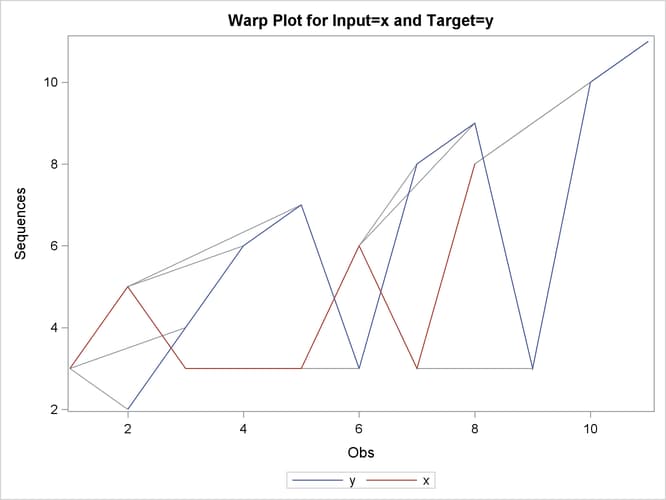
Output 31.2.16: Time Warp Plot
Output 31.2.17: Time Warp Scaled Plot
The following statements repeat the preceding similarity analysis on the example data set with warping limits:
proc similarity data=test out=_null_
   print=all plot=all;
   input x;
   target y / measure=absdev
              compress=(localabs=2)
              expand=(localabs=2);
run;
The COMPRESS=(LOCALABS=2) option limits local absolute compression to 2. The EXPAND=(LOCALABS=2) option limits local absolute expansion to 2.
Output 31.2.18: Path Plot with Warping Limits
Output 31.2.19: Warped Path Limits
Output 31.2.20: Cost Plot with Warping Limits
The following statements repeat the preceding similarity analysis on the example data set but store the results in output data sets:
proc similarity data=test out=series
   outsequence=sequences outpath=path outsum=summary;
   input x;
   target y / measure=absdev
              compress=(localabs=2)
              expand=(localabs=2);
run;
The OUT=SERIES, OUTSEQUENCE=SEQUENCES, OUTPATH=PATH, and OUTSUM=SUMMARY options specify that the output time series, time sequences, path analysis, and summary data sets be created, respectively.