The MODEL Procedure
Example 26.16 Simulated Method of Moments—AR(1) Process
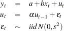
This example illustrates how to use SMM to estimate an AR(1) regression model for the following process:
In the following SAS statements,  is simulated by using this model, and the endogenous variable y is set to be equal to . The MOMENT statement creates two more moments for the estimation. One is the second moment, and the other is the first-order
autocovariance. The NPREOBS=10 option instructs PROC MODEL to run the simulation 10 times before is compared to the first observation of y. Because the initial
is simulated by using this model, and the endogenous variable y is set to be equal to . The MOMENT statement creates two more moments for the estimation. One is the second moment, and the other is the first-order
autocovariance. The NPREOBS=10 option instructs PROC MODEL to run the simulation 10 times before is compared to the first observation of y. Because the initial  is zero, the first is
  . Without the NPREOBS option, this is matched with the first observation of y. With NPREOBS, this and the next nine are thrown away, and the moment match starts with the eleventh with the first observation of y. This way, the initial values do not exert a large influence on the simulated endogenous variables.
%let nobs=500;
data ardata;
   lu =0;
   do i=-10 to &nobs;
      x = rannor( 1011 );
      e = rannor( 1011 );
      u = .6 * lu + 1.5 * e;
      Y = 2 + 1.5 * x + u;
      lu = u;
      if i > 0 then output;
   end;
run;

title1 'Simulated Method of Moments for AR(1) Process';

proc model data=ardata ;
   parms a b s 1 alpha .5;
   instrument x;

   u = alpha * zlag(u) + s * rannor( 8003 );
   ysim = a + b * x + u;
   y = ysim;
   moment y = (2) lag1(1);

   fit y / gmm npreobs=10 ndraw=10;
   bound s > 0, 1 > alpha > 0;
run;
The output of the MODEL procedure is shown in Output 26.16.1:
Output 26.16.1: PROC MODEL Output