The MODEL Procedure
Example 26.14 Simulating from a Mixture of Distributions
This example illustrates how to perform a multivariate simulation by using models that have different error distributions. Three models are used. The first model has t distributed errors. The second model is a GARCH(1,1) model with normally distributed errors. The third model has a noncentral Cauchy distribution.
The following SAS statements generate the data for this example. The t and the CAUCHY data sets use a common seed so that those two series are correlated.
/* set distribution parameters */
%let df = 7.5;
%let sig1 = .5;
%let var2 = 2.5;

data t;
   format date monyy.;
   do date='1jun2001'd  to '1nov2002'd;
              /* t-distribution with df,sig1 */
      t = .05 * date + 5000  + &sig1*tinv(ranuni(1234),&df);
      output;
   end;
run;
data normal;
   format date monyy.;
   le = &var2;
   lv = &var2;
   do date='1jun2001'd  to '1nov2002'd;
              /* Normal with GARCH error structure */
      v = 0.0001 + 0.2 * le**2 + .75 * lv;
      e = sqrt( v) * rannor(12345) ;
      normal = 25 + e;
      le = e;
      lv = v;
      output;
   end;
run;
data cauchy;
   format date monyy.;
   PI = 3.1415926;
   do date='1jun2001'd  to '1nov2002'd;
      cauchy = -4 + tan((ranuni(1234) - 0.5) * PI);
      output;
   end;
run;
Since the multivariate joint likelihood is unknown, the models must be estimated separately. The residuals for each model are saved by using the OUT= option. Also, each model is saved by using the OUTMODEL= option. The ID statement is used to provide a variable in the residual data set to merge by. The XLAG function is used to model the GARCH(1,1) process. The XLAG function returns the lag of the first argument if it is nonmissing, otherwise it returns the second argument.
title1 't-distributed Errors Example';

proc model data=t outmod=tModel;
   parms df 10 vt 4;
   t = a * date + c;
   errormodel t ~ t( vt, df );
   fit t / out=tresid;
   id date;
run;

title1 'GARCH-distributed Errors Example';

proc model data=normal outmodel=normalModel;
   normal = b0 ;
   h.normal = arch0 + arch1 * xlag(resid.normal **2 , mse.normal)
            + GARCH1 * xlag(h.normal, mse.normal);

   fit normal /fiml out=nresid;
   id date;
run;

title1 'Cauchy-distributed Errors Example';

proc model data=cauchy outmod=cauchyModel;
   parms nc = 1;
   /* nc is noncentrality parm to Cauchy dist */
   cauchy = nc;
   obj = log(1+resid.cauchy**2 * 3.1415926);
   errormodel cauchy ~ general(obj) cdf=cauchy(nc);

   fit cauchy / out=cresid;
   id date;
run;
The simulation requires a covariance matrix created from normal residuals. The following DATA step statements use the inverse CDFs of the t and Cauchy distributions to convert the residuals to the normal distribution. The CORR procedure is used to create a correlation matrix that uses the converted residuals.
/* Merge and normalize the 3 residual data sets */
data c; merge tresid nresid cresid; by date;
   t = probit(cdf("T", t/sqrt(0.2789), 16.58 ));
   cauchy = probit(cdf("CAUCHY", cauchy, -4.0623));
run;

proc corr data=c out=s;
   var t normal cauchy;
run;
Now the models can be simulated together by using the MODEL procedure SOLVE statement. The data set created by the CORR procedure is used as the correlation matrix.
title1 'Simulating Equations with Different Error Distributions';

/* Create one observation driver data set */
data sim; merge t normal cauchy; by date;
data sim; set sim(firstobs = 519 );

proc model data=sim model=( tModel normalModel cauchyModel );
   errormodel t ~ t( vt, df );
   errormodel cauchy ~ cauchy(nc);
   solve t cauchy normal / random=2000 seed=1962 out=monte
                           sdata=s(where=(_type_="CORR"));
run;
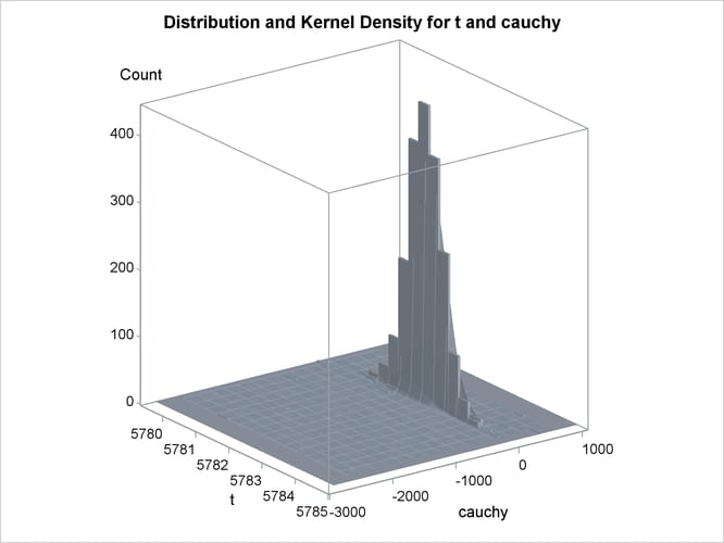
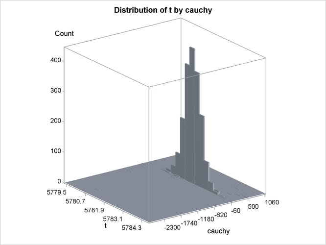
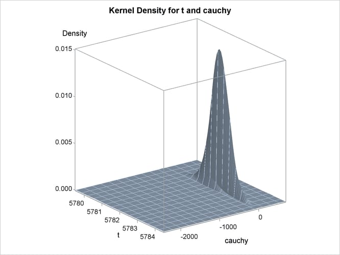
An estimation of the joint density of the t and Cauchy distribution is created by using the KDE procedure. Bounds are placed on the Cauchy dimension because of its fat tail behavior. The joint PDF is shown in Output 26.14.1.
title "T and Cauchy Distribution";

proc kde data=monte;
   univar t       / out=t_dens;
   univar cauchy  / out=cauchy_dens;
   bivar t cauchy / out=density
                    plots=all;
run;
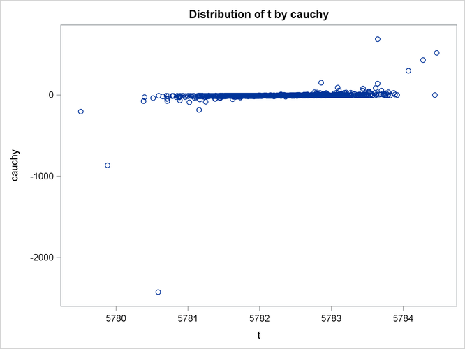
Output 26.14.1: Bivariate Density of t and Cauchy, Distribution of t by Cauchy
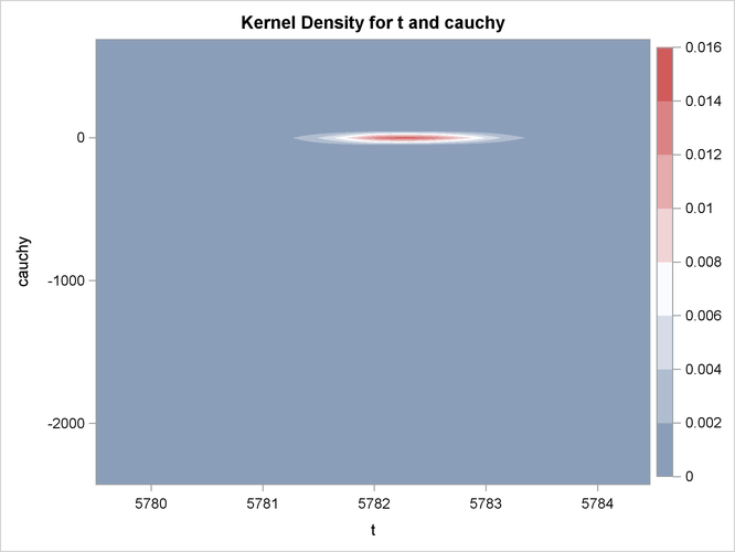
Output 26.14.2: Bivariate Density of t and Cauchy, Kernel Density for t and Cauchy
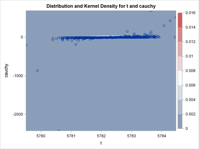
Output 26.14.3: Bivariate Density of t and Cauchy, Distribution and Kernel Density for t and Cauchy
Output 26.14.4: Bivariate Density of t and Cauchy, Distribution of t by Cauchy
Output 26.14.5: Bivariate Density of t and Cauchy, Kernel Density for t and Cauchy
Output 26.14.6: Bivariate Density of t and Cauchy, Distribution and Kernel Density for t and Cauchy