The ESM Procedure

In the previous example, the ESM procedure was used to forecast several transactional series variables by using univariate models. This example illustrates how the ESM procedure can be used to extend the independent variables that are associated with a multiple regression forecasting problem.

This example accumulates and forecasts the BOATS, CARS, and PLANES variables that were illustrated in the previous example. In addition, this example accumulates the ENGINES variable to form a time series that is then extended with missing values within the forecast horizon with the specification of MODEL=NONE.

proc esm data=websites out=nextweek lead=7;
   id time interval=dtday accumulate=total;
   forecast engines / model=none;
   forecast boats   / model=seasonal;
   forecast cars    / model=multwinters;
   forecast planes  / model=addwinters transform=log;
run;

The following AUTOREG procedure statements are used to forecast the ENGINES variable by regressing on the independent variables (BOATS, CARS, and PLANES).

proc autoreg data= nextweek;
   model engines = boats cars planes / noprint;
   output out=enginehits p=predicted;
run;

The NEXTWEEK data set created by PROC ESM is used as an input data set to PROC AUTOREG. The output data set from PROC AUTOREG contains the forecast of the variable ENGINES based on the regression model with the variables BOATS, CARS, and PLANES as regressors. See Chapter 9: The AUTOREG Procedure, for details about autoregression models.

The following statements plot the forecasts related to the ENGINES variable:

title1 "Website Data";
proc sgplot data=enginehits;
   series x=time y=boats / markers
                           markerattrs=(symbol=circlefilled color=red)
                           lineattrs=(color=red);
   series x=time y=cars / markers
                           markerattrs=(symbol=asterisk color=blue)
                           lineattrs=(color=blue);
   series x=time y=planes / markers
                           markerattrs=(symbol=circle color=styg)
                           lineattrs=(color=styg);
   scatter x=time y=predicted / markerattrs=(symbol=plus color=black);
   refline '11APR2000:00:00:00'dt / axis=x;
   xaxis values=('13MAR2000:00:00:00'dt to '18APR2000:00:00:00'dt by dtweek);
   yaxis label='Websites' minor;
run;

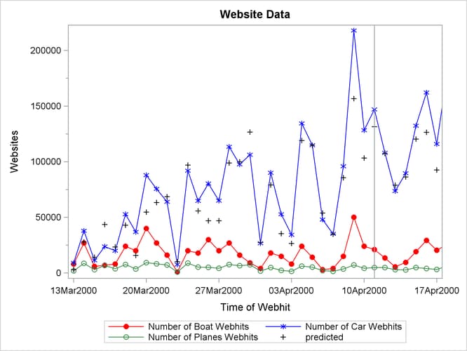
The plots are shown in Output 15.4.1. The historical data is shown to the left of the reference line and the forecasts for the next seven daily periods are shown to the right.