The SPECTRA Procedure

Example 26.1 Spectral Analysis of Sunspot Activity

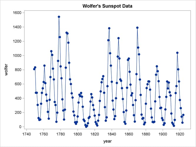
This example analyzes Wolfer’s sunspot data (Anderson, 1971). The following statements read and plot the data.

title "Wolfer's Sunspot Data";
data sunspot;
   input year wolfer @@;
datalines;
1749  809 1750  834 1751  477 1752  478 1753  307 1754  122 1755   96

   ... more lines ...

proc sgplot data=sunspot;
   series x=year y=wolfer / markers markerattrs=(symbol=circlefilled);
   xaxis values=(1740 to 1930 by 10);
   yaxis values=(0 to 1600 by 200);
run;

The plot of the sunspot series is shown in Output 26.1.1.

Output 26.1.1: Plot of Original Sunspot Data

The spectral analysis of the sunspot series is performed by the following statements:

proc spectra data=sunspot out=b p s adjmean whitetest;
   var wolfer;
   weights 1 2 3 4 3 2 1;
run;

proc print data=b(obs=12);
run;

The PROC SPECTRA statement specifies the P and S options to write the periodogram and spectral density estimates to the OUT= data set B. The WEIGHTS statement specifies a triangular spectral window for smoothing the periodogram to produce the spectral density estimate. The ADJMEAN option zeros the frequency 0 value and avoids the need to exclude that observation from the plots. The WHITETEST option prints tests for white noise.

The Fisher’s Kappa test statistic of 16.070 is larger than the 5% critical value of 7.2, so the null hypothesis that the sunspot series is white noise is rejected (see the table of critical values in Fuller (1976)).

The Bartlett’s Kolmogorov-Smirnov statistic is 0.6501, and its approximate p-value is $< 0.0001$ . The small p-value associated with this test leads to the rejection of the null hypothesis that the spectrum represents white noise.

The printed output produced by PROC SPECTRA is shown in Output 26.1.2. The output data set B created by PROC SPECTRA is shown in part in Output 26.1.3.

Output 26.1.2: White Noise Test Results

Wolfer's Sunspot Data

The SPECTRA Procedure

Test for White Noise for Variable wolfer
M-1	87
Max(P(*))	4062267
Sum(P(*))	21156512

Fisher's Kappa: (M-1)Max(P())/Sum(P(*))
Kappa	16.70489

Bartlett's Kolmogorov-Smirnov Statistic: Maximum absolute difference of the standardized partial sums of the periodogram and the CDF of a uniform(0,1) random variable.
Test Statistic	0.650055
Approximate P-Value	<.0001

Output 26.1.3: First 12 Observations of the OUT= Data Set

Wolfer's Sunspot Data

Obs	FREQ	PERIOD	P_01	S_01
1	0.00000	.	0.00	59327.52
2	0.03570	176.000	3178.15	61757.98
3	0.07140	88.000	2435433.22	69528.68
4	0.10710	58.667	1077495.76	66087.57
5	0.14280	44.000	491850.36	53352.02
6	0.17850	35.200	2581.12	36678.14
7	0.21420	29.333	181163.15	20604.52
8	0.24990	25.143	283057.60	15132.81
9	0.28560	22.000	188672.97	13265.89
10	0.32130	19.556	122673.94	14953.32
11	0.35700	17.600	58532.93	16402.84
12	0.39270	16.000	213405.16	18562.13

The following statements plot the periodogram and spectral density estimate by the frequency and period.

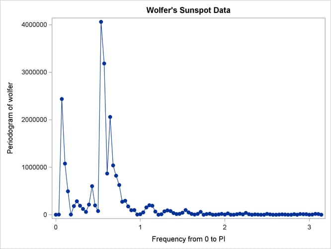
proc sgplot data=b;
   series x=freq y=p_01 / markers markerattrs=(symbol=circlefilled);
run;

proc sgplot data=b;
   series x=period y=p_01 / markers markerattrs=(symbol=circlefilled);
run;

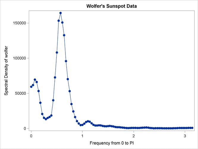
proc sgplot data=b;
   series x=freq y=s_01 / markers markerattrs=(symbol=circlefilled);
run;

proc sgplot data=b;
   series x=period y=s_01 / markers markerattrs=(symbol=circlefilled);
run;

The periodogram is plotted against the frequency in Output 26.1.4 and plotted against the period in Output 26.1.5. The spectral density estimate is plotted against the frequency in Output 26.1.6 and plotted against the period in Output 26.1.7.

Output 26.1.4: Plot of Periodogram by Frequency

Output 26.1.5: Plot of Periodogram by Period

Output 26.1.6: Plot of Spectral Density Estimate by Frequency

Output 26.1.7: Plot of Spectral Density Estimate by Period

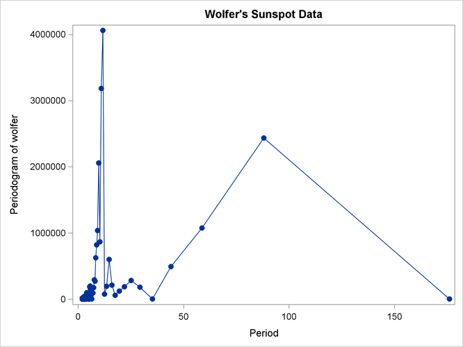
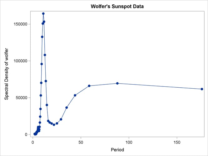
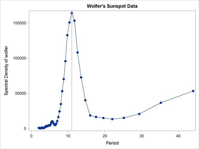
Since PERIOD is the reciprocal of frequency, the plot axis for PERIOD is stretched for low frequencies and compressed at high frequencies. One way to correct for this is to use a WHERE statement to restrict the plots and exclude the low frequency components. The following statements plot the spectral density for periods less than 50.

proc sgplot data=b;
   where period < 50;
   series x=period y=s_01 / markers markerattrs=(symbol=circlefilled);
   refline 11 / axis=x;
run;
title;

The spectral analysis of the sunspot series confirms a strong 11-year cycle of sunspot activity. The plot makes this clear by drawing a reference line at the 11 year period, which highlights the position of the main peak in the spectral density.

Output 26.1.8 shows the plot. Contrast Output 26.1.8 with Output 26.1.7.

Output 26.1.8: Plot of Spectral Density Estimate by Period to 50 Years