The FORECAST Procedure
- Overview
-
Getting Started
 Giving Dates to Forecast ValuesComputing Confidence LimitsForm of the OUT= Data SetPlotting ForecastsPlotting ResidualsModel Parameters and Goodness-of-Fit StatisticsControlling the Forecasting MethodIntroduction to Forecasting MethodsTime Trend ModelsTime Series MethodsCombining Time Trend with Autoregressive Models
 -
Syntax
-
Details
-
Examples
- References
Time trend models assume that there is some permanent deterministic pattern across time. These models are best suited to data that are not dominated by random fluctuations.
Examining a graphical plot of the time series you want to forecast is often very useful in choosing an appropriate model. The simplest case of a time trend model is one in which you assume the series is a constant plus purely random fluctuations that are independent from one time period to the next. Figure 16.8 shows how such a time series might look.
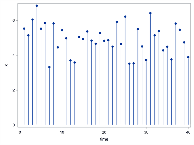
The ![]() values are generated according to the equation
values are generated according to the equation
where ![]()
![]() is an independent, zero-mean, random error and b
is an independent, zero-mean, random error and b ![]() is the true series mean.
is the true series mean.
Suppose that the series exhibits growth over time, as shown in Figure 16.9.
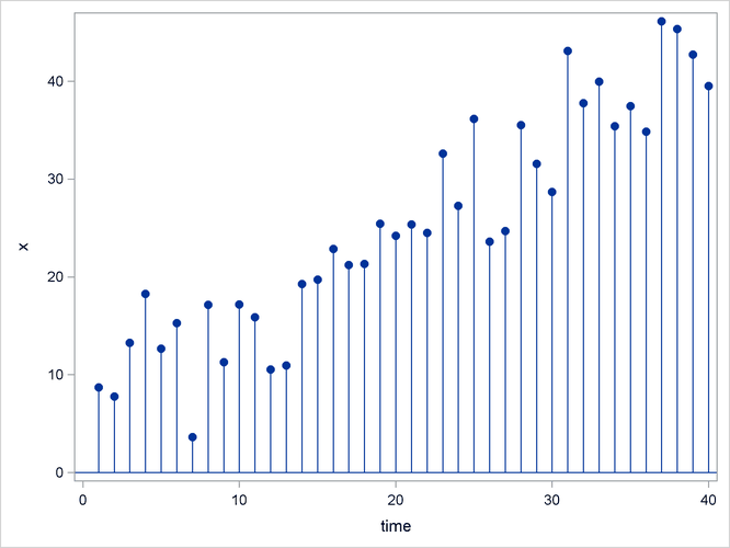
A linear model is appropriate for this data. For the linear model, assume the x ![]() values are generated according to the equation
values are generated according to the equation
The linear model has two parameters. The predicted values for the future are the points on the estimated line. The extension
of the polynomial model to three parameters is the quadratic (which forms a parabola). This allows for a constantly changing
slope, where the x ![]() values are generated according to the equation
values are generated according to the equation
PROC FORECAST can fit three types of time trend models: constant, linear, and quadratic. For other kinds of trend models, other SAS procedures can be used.
Exponential smoothing fits a time trend model by using a smoothing scheme in which the weights decline geometrically as you go backward in time. The forecasts from exponential smoothing are a time trend, but the trend is based mostly on the recent observations instead of on all the observations equally. How well exponential smoothing works as a forecasting method depends on choosing a good smoothing weight for the series.
To specify the exponential smoothing method, use the METHOD=EXPO option. Single exponential smoothing produces forecasts with a constant trend (that is, no trend). Double exponential smoothing produces forecasts with a linear trend, and triple exponential smoothing produces a quadratic trend. Use the TREND= option with the METHOD=EXPO option to select single, double, or triple exponential smoothing.
The time trend model can be modified to account for regular seasonal fluctuations of the series about the trend. To capture seasonality, the trend model includes a seasonal parameter for each season. Seasonal models can be additive or multiplicative.
where s(t) is the seasonal parameter for the season that corresponds to time t.
The Winters method is similar to exponential smoothing, but it includes seasonal factors. The Winters method can use either additive or multiplicative seasonal factors. Like exponential smoothing, good results with the Winters method depend on choosing good smoothing weights for the series to be forecast.
To specify the multiplicative or additive versions of the Winters method, use the METHOD=WINTERS or METHOD=ADDWINTERS options, respectively. To specify seasonal factors to include in the model, use the SEASONS= option.
Many observed time series do not behave like constant, linear, or quadratic time trends. However, you can partially compensate for the inadequacies of the trend models by fitting time series models to the departures from the time trend, as described in the following sections.