The X12 Procedure
- Overview
-
Getting Started

-
SyntaxFunctional SummaryPROC X12 StatementADJUST StatementARIMA StatementAUTOMDL StatementBY StatementCHECK StatementESTIMATE StatementEVENT StatementFORECAST StatementID StatementIDENTIFY StatementINPUT StatementOUTLIER StatementOUTPUT StatementPICKMDL StatementREGRESSION StatementSEATSDECOMP StatementTABLES StatementTRANSFORM StatementUSERDEFINED StatementVAR StatementX11 Statement
-
DetailsData RequirementsMissing ValuesSAS Predefined EventsUser-Defined Regression VariablesCombined Test for the Presence of Identifiable SeasonalityComputationsPICKMDL Model SelectionSEATS DecompositionDisplayed Output, ODS Table Names, and OUTPUT Tablename KeywordsUsing Auxiliary Variables to Subset Output Data SetsODS GraphicsOUT= Data SetSEATSDECOMP OUT= Data SetSpecial Data Sets
-
ExamplesARIMA Model IdentificationModel EstimationSeasonal AdjustmentRegARIMA Automatic Model SelectionAutomatic Outlier DetectionUser-Defined RegressorsMDLINFOIN= and MDLINFOOUT= Data SetsSetting Regression ParametersCreating an MDLINFO= Data Set for Use with the PICKMDL StatementIllustration of ODS GraphicsAUXDATA= Data Set
- References
This example demonstrates the use of the USERVAR= option in the REGRESSION statement to include user-defined regressors in the regARIMA model. The user-defined regressors
must be defined as nonmissing values for the span of the series being modeled plus any backcast or forecast values. Suppose
you have the data set SALESDATA with 132 monthly observations beginning in January of 1949.
title 'Data Set to be Seasonally Adjusted';
data salesdata;
   set sashelp.air(obs=132);
run;
Because the regARIMA model forecasts one year ahead, you must define the regressor for 144 observations that start in January of 1949. You can construct a simple length-of-month regressor by using the following DATA step:
title 'User-defined Regressor for Data to be Seasonally Adjusted';
data regressors(keep=date LengthOfMonth);
   set sashelp.air;
   LengthOfMonth = INTNX('MONTH',date,1) - date;
run;
In this example, the two data sets are merged to use them as input to PROC X12. You can also use the AUXDATA= data set to
input user-defined regressors. See Example 37.11 for more information. The BY statement is used to align the regressors with the time series by the time ID variable DATE.
title 'Data Set Containing Series and Regressors';
data datain;
   merge regressors salesdata;
   by date;
run;
proc print data=datain(firstobs=121);
run;
The last 24 observations of the input data set are displayed in Output 37.6.1. The regressor variable is defined for one year (12 observations) beyond the span of the time series to be seasonally adjusted.
Output 37.6.1: PROC X12 Input Data Set with User-Defined Regressor
| Data Set Containing Series and Regressors |
| Obs | DATE | LengthOfMonth | AIR |
|---|---|---|---|
| 121 | JAN59 | 31 | 360 |
| 122 | FEB59 | 28 | 342 |
| 123 | MAR59 | 31 | 406 |
| 124 | APR59 | 30 | 396 |
| 125 | MAY59 | 31 | 420 |
| 126 | JUN59 | 30 | 472 |
| 127 | JUL59 | 31 | 548 |
| 128 | AUG59 | 31 | 559 |
| 129 | SEP59 | 30 | 463 |
| 130 | OCT59 | 31 | 407 |
| 131 | NOV59 | 30 | 362 |
| 132 | DEC59 | 31 | 405 |
| 133 | JAN60 | 31 | . |
| 134 | FEB60 | 29 | . |
| 135 | MAR60 | 31 | . |
| 136 | APR60 | 30 | . |
| 137 | MAY60 | 31 | . |
| 138 | JUN60 | 30 | . |
| 139 | JUL60 | 31 | . |
| 140 | AUG60 | 31 | . |
| 141 | SEP60 | 30 | . |
| 142 | OCT60 | 31 | . |
| 143 | NOV60 | 30 | . |
| 144 | DEC60 | 31 | . |
The DATAIN data set is now ready to be used as input to PROC X12. The DATE= variable and the user-defined regressors are automatically
excluded from the variables to be seasonally adjusted.
title 'regARIMA Model with User-defined Regressor';
proc x12 data=datain date=DATE interval=MONTH plots=none;
   transform function=log;
   regression uservar=LengthOfMonth / usertype=lom;
   automdl;
   x11;
   output out=out a1 d11;
run;
The parameter estimates for the regARIMA model are shown in Output 37.6.2
Output 37.6.2: PROC X12 Output for User-Defined Regression Parameter
| regARIMA Model with User-defined Regressor |
| Regression Model Parameter Estimates | ||||||
|---|---|---|---|---|---|---|
| For Variable AIR | ||||||
| Type | Parameter | NoEst | Estimate | Standard Error | t Value | Pr > |t| |
| User Defined | LengthOfMonth | Est | 0.04683 | 0.01834 | 2.55 | 0.0119 |
| Exact ARMA Maximum Likelihood Estimation | |||||
|---|---|---|---|---|---|
| For Variable AIR | |||||
| Parameter | Lag | Estimate | Standard Error | t Value | Pr > |t| |
| Nonseasonal MA | 1 | 0.33678 | 0.08506 | 3.96 | 0.0001 |
| Seasonal MA | 12 | 0.54078 | 0.07726 | 7.00 | <.0001 |
Another way to include user-defined regressors in the regARIMA model is to specify the SPAN= option in the PROC X12 statement. The following user-defined regressor is similar to the one defined previously. However,
this length-of-month regressor is mean adjusted. Using a zero-mean regressor prevents the regressor from altering the level
of the series. In this instance, the series to be seasonally adjusted, AIR, and the regression variable, LengthOfMonth, have nonmissing observations at all time periods in the data set DATAIN.
title 'User-defined Regressor for Data to be Seasonally Adjusted, Mean Adjusted';
data datain(keep=date AIR LengthOfMonth);
   set sashelp.air;
   LengthOfMonth = INTNX('MONTH',date,1) - date - 30.4375;
run;
Because the default forecast period is one year ahead, the span of the series must be limited to one year before the end of
the regression variable definition to forecast using the regression variable LengthOfMonth,
title 'regARIMA Model with Zero-Mean User-defined Regressor';
proc x12 data=datain date=DATE interval=MONTH span=(,DEC1959) plots=none;
   transform function=log;
   regression uservar=LengthOfMonth / usertype=lom;
   automdl;
   x11;
   output out=outzm a1 d11;
run;
The parameter estimates for the regARIMA model that are estimated using a zero-mean regressor are shown in Output 37.6.3
Output 37.6.3: PROC X12 Output for Zero-Mean User-Defined Regression Parameter
| regARIMA Model with Zero-Mean User-defined Regressor |
| Regression Model Parameter Estimates | ||||||
|---|---|---|---|---|---|---|
| For Variable AIR | ||||||
| Type | Parameter | NoEst | Estimate | Standard Error | t Value | Pr > |t| |
| User Defined | LengthOfMonth | Est | 0.04683 | 0.01834 | 2.55 | 0.0119 |
| Exact ARMA Maximum Likelihood Estimation | |||||
|---|---|---|---|---|---|
| For Variable AIR | |||||
| Parameter | Lag | Estimate | Standard Error | t Value | Pr > |t| |
| Nonseasonal MA | 1 | 0.33678 | 0.08506 | 3.96 | 0.0001 |
| Seasonal MA | 12 | 0.54078 | 0.07726 | 7.00 | <.0001 |
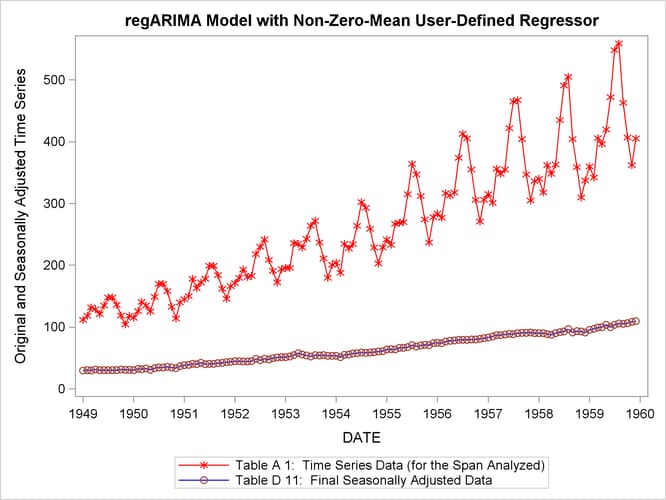
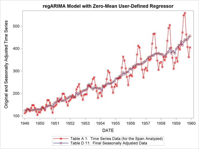
Specifying USERTYPE=LOM causes the regression effect to be removed from the seasonally adjusted series. The effect of the mean of the regression variable on the seasonally adjusted series can be seen by examining the plots of the original series and the seasonally adjusted series.
title 'regARIMA Model with Non-Zero-Mean User-Defined Regressor';
proc sgplot data=out;
   series x=date y=air_A1 / name = "A1" markers
                              markerattrs=(color=red symbol='asterisk')
                              lineattrs=(color=red);
   series x=date y=air_D11 / name= "D11" markers
                               markerattrs=(symbol='circle')
                               lineattrs=(color=blue);
   yaxis label='Original and Seasonally Adjusted Time Series';
run;
title 'regARIMA Model with Zero-Mean User-Defined Regressor';
proc sgplot data=outzm;
   series x=date y=air_A1 / name = "A1" markers
                              markerattrs=(color=red symbol='asterisk')
                              lineattrs=(color=red);
   series x=date y=air_D11 / name= "D11" markers
                               markerattrs=(symbol='circle')
                               lineattrs=(color=blue);
   yaxis label='Original and Seasonally Adjusted Time Series';
run;
The graph of the original and seasonally adjusted series in Output 37.6.4 shows that the level of the seasonally adjusted series has been altered due to the user-defined regressor. The graph of the original and seasonally adjusted series in Output 37.6.5 shows that the level of the seasonally adjusted series is the same as the original series since the user-defined regressor has zero-mean.
When actual values are available for the forecast periods, information about forecast error is available in the output. Output 37.6.6 shows the table “Forecasts and Standard Errors of the Transformed Data on the Original Scale” for a series with missing values in the forecast period. Output 37.6.7 shows the table “Forecasts and Standard Errors of the Transformed Data on the Original Scale” for a series with actual values in the forecast period. Thus, it is more desirable to use SPAN= option to limit the span of a series if the actual values are available for the forecast period.
Output 37.6.6: PROC X12 Forecasts for Series Extended with Missing Values
| Forecasts and Standard Errors of the Transformed Data |
||||
|---|---|---|---|---|
| On the Original scale | ||||
| For Variable AIR | ||||
| Date | Forecast | Standard Error | 95% Confidence Limits | |
| JAN1960 | 419.600 | 14.85053 | 391.509 | 449.705 |
| FEB1960 | 416.480 | 19.05188 | 380.826 | 455.472 |
| MAR1960 | 466.697 | 22.66762 | 424.402 | 513.208 |
| APR1960 | 454.468 | 24.53242 | 408.951 | 505.051 |
| MAY1960 | 473.876 | 27.91366 | 422.353 | 531.684 |
| JUN1960 | 547.601 | 34.74893 | 483.769 | 619.855 |
| JUL1960 | 623.318 | 42.20549 | 546.139 | 711.405 |
| AUG1960 | 631.731 | 45.30824 | 549.231 | 726.623 |
| SEP1960 | 527.221 | 39.81839 | 455.011 | 610.890 |
| OCT1960 | 462.774 | 36.63020 | 396.605 | 539.984 |
| NOV1960 | 407.155 | 33.64286 | 346.608 | 478.277 |
| DEC1960 | 452.702 | 38.91914 | 382.913 | 535.212 |
Output 37.6.7: PROC X12 Forecasts for Series with Actual Values in Forecast Periods
| Forecasts and Standard Errors of the Transformed Data | |||||||
|---|---|---|---|---|---|---|---|
| On the Original scale | |||||||
| For Variable AIR | |||||||
| Date | Data | Forecast | Forecast Error | Standard Error | t Value | 95% Confidence Limits | |
| JAN1960 | 417.000 | 419.600 | -2.600 | 14.85053 | -0.18 | 391.509 | 449.705 |
| FEB1960 | 391.000 | 416.480 | -25.480 | 19.05188 | -1.34 | 380.826 | 455.472 |
| MAR1960 | 419.000 | 466.697 | -47.697 | 22.66762 | -2.10 | 424.402 | 513.208 |
| APR1960 | 461.000 | 454.468 | 6.532 | 24.53242 | 0.27 | 408.951 | 505.051 |
| MAY1960 | 472.000 | 473.876 | -1.876 | 27.91366 | -0.07 | 422.353 | 531.684 |
| JUN1960 | 535.000 | 547.601 | -12.601 | 34.74893 | -0.36 | 483.769 | 619.855 |
| JUL1960 | 622.000 | 623.318 | -1.318 | 42.20549 | -0.03 | 546.139 | 711.405 |
| AUG1960 | 606.000 | 631.731 | -25.731 | 45.30824 | -0.57 | 549.231 | 726.623 |
| SEP1960 | 508.000 | 527.221 | -19.221 | 39.81839 | -0.48 | 455.011 | 610.890 |
| OCT1960 | 461.000 | 462.774 | -1.774 | 36.63020 | -0.05 | 396.605 | 539.984 |
| NOV1960 | 390.000 | 407.155 | -17.155 | 33.64286 | -0.51 | 346.608 | 478.277 |
| DEC1960 | 432.000 | 452.702 | -20.702 | 38.91914 | -0.53 | 382.913 | 535.212 |