The STATESPACE Procedure

The STATESPACE procedure is designed to automatically select the best state space model for forecasting the series. You can specify your own model if you want, and you can use the output from PROC STATESPACE to help you identify a state space model. However, the easiest way to use PROC STATESPACE is to let it choose the model.
Although PROC STATESPACE selects the state space model automatically, it does assume that the input series are stationary. If the series are nonstationary, then the process might fail. Therefore the first step is to examine your data and test to see if differencing is required. (See the section Stationarity and Differencing for further discussion of this issue.)
The series shown in Figure 28.1 are nonstationary. In order to forecast X and Y with a state space model, you must difference them (or use some other detrending method). If you fail to difference when needed and try to use PROC STATESPACE with nonstationary data, an inappropriate state space model might be selected, and the model estimation might fail to converge.
The following statements identify and fit a state space model for the first differences of X and Y, and forecast X and Y 10 periods ahead:
proc statespace data=in out=out lead=10;
   var x(1) y(1);
   id t;
run;
The DATA= option specifies the input data set and the OUT= option specifies the output data set for the forecasts. The LEAD= option specifies forecasting 10 observations past the end of the input data. The VAR statement specifies the variables to forecast and specifies differencing. The notation X(1) Y(1) specifies that the state space model analyzes the first differences of X and Y.
The first page of the printed output produced by the preceding statements is shown in Figure 28.2.
Figure 28.2: Descriptive Statistics and VAR Order Selection
| Number of Observations | 200 |
|---|
| Variable | Mean | Standard Error | |
|---|---|---|---|
| x | 0.144316 | 1.233457 | Has been differenced. With period(s) = 1. |
| y | 0.164871 | 1.304358 | Has been differenced. With period(s) = 1. |
| Information Criterion for Autoregressive Models | ||||||||||
|---|---|---|---|---|---|---|---|---|---|---|
| Lag=0 | Lag=1 | Lag=2 | Lag=3 | Lag=4 | Lag=5 | Lag=6 | Lag=7 | Lag=8 | Lag=9 | Lag=10 |
| 149.697 | 8.387786 | 5.517099 | 12.05986 | 15.36952 | 21.79538 | 24.00638 | 29.88874 | 33.55708 | 41.17606 | 47.70222 |
| Schematic Representation of Correlations | |||||||||||
|---|---|---|---|---|---|---|---|---|---|---|---|
| Name/Lag | 0 | 1 | 2 | 3 | 4 | 5 | 6 | 7 | 8 | 9 | 10 |
| x | ++ | ++ | ++ | ++ | ++ | ++ | +. | .. | +. | +. | .. |
| y | ++ | ++ | ++ | ++ | ++ | +. | +. | +. | +. | .. | .. |
| + is > 2*std error, - is < -2*std error, . is between | |||||||||||
Descriptive statistics are printed first, giving the number of nonmissing observations after differencing and the sample means and standard deviations of the differenced series. The sample means are subtracted before the series are modeled (unless the NOCENTER option is specified), and the sample means are added back when the forecasts are produced.
Let ![]() and
and ![]() be the observed values of X and Y, and let
be the observed values of X and Y, and let ![]() and
and ![]() be the values of X and Y after differencing and subtracting the mean difference. The series
be the values of X and Y after differencing and subtracting the mean difference. The series ![]() modeled by the STATEPSPACE procedure is
modeled by the STATEPSPACE procedure is
where B represents the backshift operator.
After the descriptive statistics, PROC STATESPACE prints the Akaike information criterion (AIC) values for the autoregressive models fit to the series. The smallest AIC value, in this case 5.517 at lag 2, determines the number of autocovariance matrices analyzed in the canonical correlation phase.
A schematic representation of the autocorrelations is printed next. This indicates which elements of the autocorrelation matrices at different lags are significantly greater than or less than 0.
The second page of the STATESPACE printed output is shown in Figure 28.3.
Figure 28.3: Partial Autocorrelations and VAR Model
| Schematic Representation of Partial Autocorrelations |
||||||||||
|---|---|---|---|---|---|---|---|---|---|---|
| Name/Lag | 1 | 2 | 3 | 4 | 5 | 6 | 7 | 8 | 9 | 10 |
| x | ++ | +. | .. | .. | .. | .. | .. | .. | .. | .. |
| y | ++ | .. | .. | .. | .. | .. | .. | .. | .. | .. |
| + is > 2*std error, - is < -2*std error, . is between | ||||||||||
| Yule-Walker Estimates for Minimum AIC | ||||
|---|---|---|---|---|
| Lag=1 | Lag=2 | |||
| x | y | x | y | |
| x | 0.257438 | 0.202237 | 0.170812 | 0.133554 |
| y | 0.292177 | 0.469297 | -0.00537 | -0.00048 |
Figure 28.3 shows a schematic representation of the partial autocorrelations, similar to the autocorrelations shown in Figure 28.2. The selection of a second order autoregressive model by the AIC statistic looks reasonable in this case because the partial autocorrelations for lags greater than 2 are not significant.
Next, the Yule-Walker estimates for the selected autoregressive model are printed. This output shows the coefficient matrices of the vector autoregressive model at each lag.
After the autoregressive order selection process has determined the number of lags to consider, the canonical correlation analysis phase selects the state vector. By default, output for this process is not printed. You can use the CANCORR option to print details of the canonical correlation analysis. See the section Canonical Correlation Analysis Options for an explanation of this process.
After the state vector is selected, the state space model is estimated by approximate maximum likelihood. Information from the canonical correlation analysis and from the preliminary autoregression is used to form preliminary estimates of the state space model parameters. These preliminary estimates are used as starting values for the iterative estimation process.
The form of the state vector and the preliminary estimates are printed next, as shown in Figure 28.4.
Figure 28.4: Preliminary Estimates of State Space Model
| State Vector | ||
|---|---|---|
| x(T;T) | y(T;T) | x(T+1;T) |
| Estimate of Transition Matrix | ||
|---|---|---|
| 0 | 0 | 1 |
| 0.291536 | 0.468762 | -0.00411 |
| 0.24869 | 0.24484 | 0.204257 |
| Input Matrix for Innovation | |
|---|---|
| 1 | 0 |
| 0 | 1 |
| 0.257438 | 0.202237 |
| Variance Matrix for Innovation | |
|---|---|
| 0.945196 | 0.100786 |
| 0.100786 | 1.014703 |
Figure 28.4 first prints the state vector as X[T;T] Y[T;T] X[T+1;T]. This notation indicates that the state vector is
![\begin{eqnarray*} \Strong{z}_{t} = \left[\begin{matrix} x_{t|t} \\ y_{t|t} \\ x_{t+1|t} \end{matrix}\right] \nonumber \end{eqnarray*}](images/etsug_statespa0029.png)
The notation ![]() indicates the conditional expectation or prediction of
indicates the conditional expectation or prediction of ![]() based on the information available at time t, and
based on the information available at time t, and ![]() and
and ![]() are
are ![]() and
and ![]() , respectively.
, respectively.
The remainder of Figure 28.4 shows the preliminary estimates of the transition matrix ![]() , the input matrix
, the input matrix ![]() , and the covariance matrix
, and the covariance matrix ![]() .
.
The next page of the STATESPACE output prints the final estimates of the fitted model, as shown in Figure 28.5. This output has the same form as in Figure 28.4, but it shows the maximum likelihood estimates instead of the preliminary estimates.
Figure 28.5: Fitted State Space Model
| State Vector | ||
|---|---|---|
| x(T;T) | y(T;T) | x(T+1;T) |
| Estimate of Transition Matrix | ||
|---|---|---|
| 0 | 0 | 1 |
| 0.297273 | 0.47376 | -0.01998 |
| 0.2301 | 0.228425 | 0.256031 |
| Input Matrix for Innovation | |
|---|---|
| 1 | 0 |
| 0 | 1 |
| 0.257284 | 0.202273 |
| Variance Matrix for Innovation | |
|---|---|
| 0.945188 | 0.100752 |
| 0.100752 | 1.014712 |
The estimated state space model shown in Figure 28.5 is
![\begin{eqnarray*} \left[\begin{matrix} x_{t+1|t+1} \\ y_{t+1|t+1} \\ x_{t+2|t+1} \end{matrix}\right] & =& \left[\begin{matrix} 0 & 0 & 1 \\ 0.297 & 0.474 & -0.020 \\ 0.230 & 0.228 & 0.256 \end{matrix}\right] \left[\begin{matrix} x_{t} \\ y_{t} \\ x_{t+1|t} \end{matrix}\right] + \left[\begin{matrix} 1 & 0 \\ 0 & 1 \\ 0.257 & 0.202 \end{matrix}\right] \left[\begin{matrix} e_{t+1} \\ n_{t+1} \end{matrix}\right] \\ {var}\left[\begin{matrix} e_{t+1} \\ n_{t+1} \end{matrix}\right] & =& \left[\begin{matrix} 0.945 & 0.101 \\ 0.101 & 1.015 \end{matrix}\right] \nonumber \end{eqnarray*}](images/etsug_statespa0035.png)
The next page of the STATESPACE output lists the estimates of the free parameters in the ![]() and
and ![]() matrices with standard errors and t statistics, as shown in Figure 28.6.
matrices with standard errors and t statistics, as shown in Figure 28.6.
Figure 28.6: Final Parameter Estimates
| Parameter Estimates | |||
|---|---|---|---|
| Parameter | Estimate | Standard Error | t Value |
| F(2,1) | 0.297273 | 0.129995 | 2.29 |
| F(2,2) | 0.473760 | 0.115688 | 4.10 |
| F(2,3) | -0.01998 | 0.313025 | -0.06 |
| F(3,1) | 0.230100 | 0.126226 | 1.82 |
| F(3,2) | 0.228425 | 0.112978 | 2.02 |
| F(3,3) | 0.256031 | 0.305256 | 0.84 |
| G(3,1) | 0.257284 | 0.071060 | 3.62 |
| G(3,2) | 0.202273 | 0.068593 | 2.95 |
The maximum likelihood estimates are computed by an iterative nonlinear maximization algorithm, which might not converge. If the estimates fail to converge, warning messages are printed in the output.
If you encounter convergence problems, you should recheck the stationarity of the data and ensure that the specified differencing orders are correct. Attempting to fit state space models to nonstationary data is a common cause of convergence failure. You can also use the MAXIT= option to increase the number of iterations allowed, or experiment with the convergence tolerance options DETTOL= and PARMTOL=.
The following statements print the output data set. The WHERE statement excludes the first 190 observations from the output, so that only the forecasts and the last 10 actual observations are printed.
proc print data=out;
   id t;
   where t > 190;
run;
The PROC PRINT output is shown in Figure 28.7.
Figure 28.7: OUT= Data Set Produced by PROC STATESPACE
| t | x | FOR1 | RES1 | STD1 | y | FOR2 | RES2 | STD2 |
|---|---|---|---|---|---|---|---|---|
| 191 | 34.8159 | 33.6299 | 1.18600 | 0.97221 | 58.7189 | 57.9916 | 0.72728 | 1.00733 |
| 192 | 35.0656 | 35.6598 | -0.59419 | 0.97221 | 58.5440 | 59.7718 | -1.22780 | 1.00733 |
| 193 | 34.7034 | 35.5530 | -0.84962 | 0.97221 | 59.0476 | 58.5723 | 0.47522 | 1.00733 |
| 194 | 34.6626 | 34.7597 | -0.09707 | 0.97221 | 59.7774 | 59.2241 | 0.55330 | 1.00733 |
| 195 | 34.4055 | 34.8322 | -0.42664 | 0.97221 | 60.5118 | 60.1544 | 0.35738 | 1.00733 |
| 196 | 33.8210 | 34.6053 | -0.78434 | 0.97221 | 59.8750 | 60.8260 | -0.95102 | 1.00733 |
| 197 | 34.0164 | 33.6230 | 0.39333 | 0.97221 | 58.4698 | 59.4502 | -0.98046 | 1.00733 |
| 198 | 35.3819 | 33.6251 | 1.75684 | 0.97221 | 60.6782 | 57.9167 | 2.76150 | 1.00733 |
| 199 | 36.2954 | 36.0528 | 0.24256 | 0.97221 | 60.9692 | 62.1637 | -1.19450 | 1.00733 |
| 200 | 37.8945 | 37.1431 | 0.75142 | 0.97221 | 60.8586 | 61.4085 | -0.54984 | 1.00733 |
| 201 | . | 38.5068 | . | 0.97221 | . | 61.3161 | . | 1.00733 |
| 202 | . | 39.0428 | . | 1.59125 | . | 61.7509 | . | 1.83678 |
| 203 | . | 39.4619 | . | 2.28028 | . | 62.1546 | . | 2.62366 |
| 204 | . | 39.8284 | . | 2.97824 | . | 62.5099 | . | 3.38839 |
| 205 | . | 40.1474 | . | 3.67689 | . | 62.8275 | . | 4.12805 |
| 206 | . | 40.4310 | . | 4.36299 | . | 63.1139 | . | 4.84149 |
| 207 | . | 40.6861 | . | 5.03040 | . | 63.3755 | . | 5.52744 |
| 208 | . | 40.9185 | . | 5.67548 | . | 63.6174 | . | 6.18564 |
| 209 | . | 41.1330 | . | 6.29673 | . | 63.8435 | . | 6.81655 |
| 210 | . | 41.3332 | . | 6.89383 | . | 64.0572 | . | 7.42114 |
The OUT= data set produced by PROC STATESPACE contains the VAR and ID statement variables. In addition, for each VAR statement variable, the OUT= data set contains the variables FORi, RESi, and STDi. These variables contain the predicted values, residuals, and forecast standard errors for the ith variable in the VAR statement list. In this case, X is listed first in the VAR statement, so FOR1 contains the forecasts of X, while FOR2 contains the forecasts of Y.
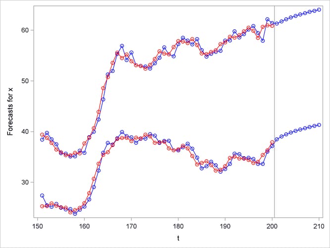
The following statements plot the forecasts and actuals for the series.
proc sgplot data=out noautolegend;
   where t > 150;
   series x=t y=for1 / markers
    markerattrs=(symbol=circle color=blue)
    lineattrs=(pattern=solid color=blue);
  series x=t y=for2 / markers
   markerattrs=(symbol=circle color=blue)
   lineattrs=(pattern=solid color=blue);
  series x=t y=x / markers
   markerattrs=(symbol=circle color=red)
   lineattrs=(pattern=solid color=red);
  series x=t y=y / markers
   markerattrs=(symbol=circle color=red)
   lineattrs=(pattern=solid color=red);
  refline 200.5 / axis=x;
run;
The forecast plot is shown in Figure 28.8. The last 50 observations are also plotted to provide context, and a reference line is drawn between the historical and forecast periods.
By default, the STATESPACE procedure produces a large amount of printed output. The NOPRINT option suppresses all printed output. You can suppress the printed output for the autoregressive model selection process with the PRINTOUT=NONE option. The descriptive statistics and state space model estimation output are still printed when PRINTOUT=NONE is specified. You can produce more detailed output with the PRINTOUT=LONG option and by specifying the printing control options CANCORR, COVB, and PRINT.