The PANEL Procedure
- Overview
- Getting Started
-
Syntax

-
DetailsSpecifying the Input DataSpecifying the Regression ModelUnbalanced DataMissing ValuesComputational ResourcesRestricted EstimatesNotationOne-Way Fixed-Effects ModelTwo-Way Fixed-Effects ModelBalanced PanelsUnbalanced PanelsBetween EstimatorsPooled EstimatorOne-Way Random-Effects ModelTwo-Way Random-Effects ModelParks Method (Autoregressive Model)Da Silva Method (Variance-Component Moving Average Model)Dynamic Panel EstimatorLinear Hypothesis TestingHeteroscedasticity-Corrected Covariance MatricesHeteroscedasticity- and Autocorrelation-Consistent Covariance MatricesR-SquareSpecification TestsPanel Data Poolability TestPanel Data Unit Root TestsTroubleshootingCreating ODS GraphicsOUTPUT OUT= Data SetOUTEST= Data SetOUTTRANS= Data SetPrinted OutputODS Table Names
-
Example
- References
Levin, Lin, and Chu (2002)
Levin, Lin, and Chu (2002) propose a panel unit root test for the null hypothesis of unit root against a homogeneous stationary hypothesis. The model is specified as
Three models are considered: (1) ![]() (the empty set) with no individual effects, (2)
(the empty set) with no individual effects, (2) ![]() in which the series
in which the series ![]() has an individual-specific mean but no time trend, and (3)
has an individual-specific mean but no time trend, and (3) ![]() in which the series
in which the series ![]() has an individual-specific mean and linear and individual-specific time trend. The panel unit root test evaluates the null
hypothesis of
has an individual-specific mean and linear and individual-specific time trend. The panel unit root test evaluates the null
hypothesis of ![]() , for all
, for all ![]() , against the alternative hypothesis
, against the alternative hypothesis ![]() for all
for all ![]() . The lag order
. The lag order ![]() is unknown and is allowed to vary across individuals. It can be selected by the methods that are described in the section
Lag Order Selection in the ADF Regression. Denote the selected lag orders as
is unknown and is allowed to vary across individuals. It can be selected by the methods that are described in the section
Lag Order Selection in the ADF Regression. Denote the selected lag orders as ![]() . The test is implemented in three steps.
. The test is implemented in three steps.
- Step 1
-
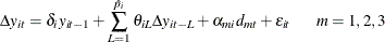
The ADF regressions are implemented for each individual
 , and then the orthogonalized residuals are generated and normalized. That is, the following model is estimated:
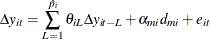
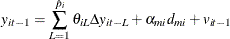
The two orthogonalized residuals are generated by the following two auxiliary regressions:
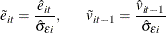
The residuals are saved at
 and
and  , respectively. To remove heteroscedasticity, the residuals and are normalized by the regression standard error from the ADF regression. Denote the standard error as
 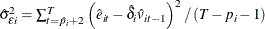 , and normalize residuals as
- Step 2
-
The ratios of long-run to short-run standard deviations of
 are estimated. Denote the ratios and the long-run variances as
  and
and  , respectively. The long-run variances are estimated by the HAC (heteroscedasticity- and autocorrelation-consistent) estimators,
which are described in the section Long-Run Variance Estimation. Then the ratios are estimated by
, respectively. The long-run variances are estimated by the HAC (heteroscedasticity- and autocorrelation-consistent) estimators,
which are described in the section Long-Run Variance Estimation. Then the ratios are estimated by  . Let the average standard deviation ratio be
 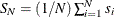 , and let its estimator be
 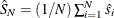 .
. - Step 3
-
The panel test statistics are calculated. To calculate the t statistic and the adjusted t statistic, the following equation is estimated:
The total number of observations is
 , with
  . The standard t statistic for testing
  is
is  , with OLS estimator
  and standard deviation
  . However, the standard t statistic diverges to negative infinity for models (2) and (3). Let
  be the root mean square error from the step 3 regression, and denote it as
![\begin{equation*} \hat{\sigma }_{\tilde{\varepsilon }}^{2} = \left[\frac{1}{N\tilde{T}}\sum _{i=1}^{N}\sum _{t=2+\hat{p}_{i}}^{T}(\tilde{e}_{it}-\hat{\delta }\tilde{v}_{it-1})^{2}\right] \end{equation*}](images/etsug_panel0720.png)
Levin, Lin, and Chu (2002) propose the following adjusted t statistic:
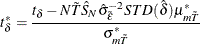
The mean and standard deviation adjustments (
 ) depend on the time series dimension
  and model specification
  , which can be found in Table 2 of Levin, Lin, and Chu (2002). The adjusted t statistic converges to the standard normal distribution. Therefore, the standard normal critical values are used in hypothesis
testing.
, which can be found in Table 2 of Levin, Lin, and Chu (2002). The adjusted t statistic converges to the standard normal distribution. Therefore, the standard normal critical values are used in hypothesis
testing.
The methods for selecting the individual lag orders in the ADF regressions can be divided into two categories: selection based on information criteria and selection via sequential testing.
In this method, the following information criteria can be applied to lag order selection: AIC, SBC, HQIC (HQC), and MAIC.
As with other model selection applications, the lag order is selected from 0 to the maximum ![]() to minimize the objective function, plus a penalty term, which is a function of the number of parameters in the regression.
Let
to minimize the objective function, plus a penalty term, which is a function of the number of parameters in the regression.
Let ![]() be the number of parameters and
be the number of parameters and ![]() be the number of effective observations. For regression models, the objective function is
be the number of effective observations. For regression models, the objective function is ![]() , where SSR is the sum of squared residuals. For AIC, the penalty term equals
, where SSR is the sum of squared residuals. For AIC, the penalty term equals ![]() . For SBC, this term is
. For SBC, this term is ![]() . For HQIC, it is
. For HQIC, it is ![]() with
with ![]() being a constant greater than 1.[7] For MAIC, the penalty term equals
being a constant greater than 1.[7] For MAIC, the penalty term equals ![]() , where
, where
and ![]() is the estimated coefficient of the lagged dependent variable
is the estimated coefficient of the lagged dependent variable ![]() in the ADF regression.
in the ADF regression.
In this method, the lag order estimation is based on the statistical significance of the estimated AR coefficients. Hall
(1994) proposed general-to-specific (GS) and specific-to-general (SG) strategies. Levin, Lin, and Chu (2002) recommend the first strategy, following Campbell and Perron (1991). In the GS modeling strategy, starting with the maximum lag order ![]() , the t test for the largest lag order in
, the t test for the largest lag order in ![]() is performed to determine whether a smaller lag order is preferred. Specifically, when the null of
is performed to determine whether a smaller lag order is preferred. Specifically, when the null of ![]() is not rejected given the significance level (
is not rejected given the significance level (![]() ), a smaller lag order is preferred. This procedure continues until a statistically significant lag order is reached. On the
other hand, the SG modeling strategy starts with lag order 0 and moves toward the maximum lag order
), a smaller lag order is preferred. This procedure continues until a statistically significant lag order is reached. On the
other hand, the SG modeling strategy starts with lag order 0 and moves toward the maximum lag order ![]() .
.
The long-run variance of ![]() is estimated by a HAC-type estimator. For model (1), given the lag truncation parameter
is estimated by a HAC-type estimator. For model (1), given the lag truncation parameter ![]() and kernel weights
and kernel weights ![]() , the formula is
, the formula is
To achieve consistency, the lag truncation parameter must satisfy ![]() and
and ![]() as
as ![]() . Levin, Lin, and Chu (2002) suggest
. Levin, Lin, and Chu (2002) suggest ![]() . The weights
. The weights ![]() depend on the kernel function. Andrews (1991) proposes data-driven bandwidth (lag truncation parameter + 1 if integer-valued) selection procedures to minimize the asymptotic
mean squared error (MSE) criterion. For details about the kernel functions and Andrews (1991) data-driven bandwidth selection procedure, see the section Heteroscedasticity- and Autocorrelation-Consistent Covariance Matrices for details. Because Levin, Lin, and Chu (2002) truncate the bandwidth as an integer, when LLCBAND is specified as the BANDWIDTH option, it corresponds to
depend on the kernel function. Andrews (1991) proposes data-driven bandwidth (lag truncation parameter + 1 if integer-valued) selection procedures to minimize the asymptotic
mean squared error (MSE) criterion. For details about the kernel functions and Andrews (1991) data-driven bandwidth selection procedure, see the section Heteroscedasticity- and Autocorrelation-Consistent Covariance Matrices for details. Because Levin, Lin, and Chu (2002) truncate the bandwidth as an integer, when LLCBAND is specified as the BANDWIDTH option, it corresponds to ![]() . Furthermore, kernel weights
. Furthermore, kernel weights ![]() with kernel function
with kernel function ![]() .
.
For model (2), the series ![]() is demeaned individual by individual first. Therefore,
is demeaned individual by individual first. Therefore, ![]() is replaced by
is replaced by ![]() , where
, where ![]() is the mean of
is the mean of ![]() for individual
for individual ![]() . For model (3) with individual fixed effects and time trend, both the individual mean and trend should be removed before
the long-run variance is estimated. That is, first regress
. For model (3) with individual fixed effects and time trend, both the individual mean and trend should be removed before
the long-run variance is estimated. That is, first regress ![]() on
on ![]() for each individual and save the residual
for each individual and save the residual ![]() , and then replace
, and then replace ![]() with the residual.
with the residual.
The Levin, Lin, and Chu (2002) testing procedure is based on the assumption of cross-sectional independence. It is possible to relax this assumption and
allow for a limited degree of dependence via time-specific aggregate effects. Let ![]() denote the time-specific aggregate effects; then the data generating process (DGP) becomes
denote the time-specific aggregate effects; then the data generating process (DGP) becomes
By subtracting the cross-sectional averages ![]() from the observed dependent variable
from the observed dependent variable ![]() , or equivalently, by including the time-specific intercepts
, or equivalently, by including the time-specific intercepts ![]() in the ADF regression, the cross-sectional dependence is removed. The impact of a single aggregate common factor that has an identical
impact on all individuals but changes over time can also be removed in this way. After cross-sectional dependence is removed,
the three-step procedure is applied to calculate the Levin, Lin, and Chu (2002) adjusted t statistic.
in the ADF regression, the cross-sectional dependence is removed. The impact of a single aggregate common factor that has an identical
impact on all individuals but changes over time can also be removed in this way. After cross-sectional dependence is removed,
the three-step procedure is applied to calculate the Levin, Lin, and Chu (2002) adjusted t statistic.
Three deterministic variables can be included in the model for the first-stage estimation: CS_FixedEffects (cross-sectional fixed effects), TS_FixedEffects (time series fixed effects), and TimeTrend (individual linear time trend). When a linear time trend is included, the individual fixed effects are also included. Otherwise the time trend is not identified. Moreover, if the time fixed effects are included, the time trend is not identified either. Therefore, we have 5 identified models: model (1), no deterministic variables; model (2), CS_FixedEffects; model (3), CS_FixedEffects and TimeTrend; model (4), TS_FixedEffects; model (5), CS_FixedEffects TS_FixedEffects. PROC PANEL outputs the test results for all 5 model specifications.
Im, Pesaran, and Shin (2003)
To test for the unit root in heterogeneous panels, Im, Pesaran, and Shin (2003) propose a standardized ![]() -bar test statistic based on averaging the (augmented) Dickey-Fuller statistics across the groups. The limiting distribution
is standard normal. The stochastic process
-bar test statistic based on averaging the (augmented) Dickey-Fuller statistics across the groups. The limiting distribution
is standard normal. The stochastic process ![]() is generated by the first-order autoregressive process. If
is generated by the first-order autoregressive process. If ![]() , the data generating process can be expressed as in LLC:
, the data generating process can be expressed as in LLC:
Unlike the DGP in LLC, ![]() is allowed to differ across groups. The null hypothesis of unit roots is
is allowed to differ across groups. The null hypothesis of unit roots is
against the heterogeneous alternative,
The Im, Pesaran, and Shin test also allows for some (but not all) of the individual series to have unit roots under the alternative
hypothesis. But the fraction of the individual processes that are stationary is positive, ![]() . The
. The ![]() -bar statistic, denoted by
-bar statistic, denoted by ![]() , is formed as a simple average of the individual t statistics for testing the null hypothesis of
, is formed as a simple average of the individual t statistics for testing the null hypothesis of ![]() . If
. If ![]() is the standard t statistic, then
is the standard t statistic, then
If ![]() , then for each
, then for each ![]() the t statistic (without time trend) converges to the Dickey-Fuller distribution,
the t statistic (without time trend) converges to the Dickey-Fuller distribution, ![]() , defined by
, defined by
where ![]() is the standard Brownian motion. The limiting distribution is different when a time trend is included in the regression (Hamilton,
1994, p. 499). The mean and variance of the limiting distributions are reported in Nabeya (1999). The standardized
is the standard Brownian motion. The limiting distribution is different when a time trend is included in the regression (Hamilton,
1994, p. 499). The mean and variance of the limiting distributions are reported in Nabeya (1999). The standardized ![]() -bar statistic satisfies
-bar statistic satisfies
where the standard normal is the sequential limit with ![]() followed by
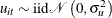
followed by ![]() . To obtain better finite sample approximations, Im, Pesaran, and Shin (2003) propose standardizing the
. To obtain better finite sample approximations, Im, Pesaran, and Shin (2003) propose standardizing the ![]() -bar statistic by means and variances of
-bar statistic by means and variances of ![]() under the null hypothesis
under the null hypothesis ![]() . The alternative standardized
. The alternative standardized ![]() -bar statistic is
-bar statistic is
![\begin{equation*} W_{tbar}(p, \rho ) = \frac{\sqrt {N} \{ t\text {-bar}_{NT} - \sum _{i = 1}^{N}E[t_{iT}(p_{i}, 0)| \beta _{i} = 0] /N\} }{\sqrt {\sum _{i = 1}^{N}Var[t_{iT}(p_{i}, 0)| \beta _{i} = 0]/N}}\implies \mathcal{N}(0,1) \end{equation*}](images/etsug_panel0771.png)
Im, Pesaran, and Shin (2003) simulate the values of ![]() and
and ![]() for different values of
for different values of ![]() and
and ![]() . The lag order in the ADF regression can be selected by the same method as in Levin, Lin, and Chu (2002). See the section Lag Order Selection in the ADF Regression for details.
. The lag order in the ADF regression can be selected by the same method as in Levin, Lin, and Chu (2002). See the section Lag Order Selection in the ADF Regression for details.
When ![]() is fixed, Im, Pesaran, and Shin (2003) assume serially uncorrelated errors,
is fixed, Im, Pesaran, and Shin (2003) assume serially uncorrelated errors, ![]() ;
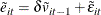
; ![]() is likely to have finite second moment, which is not established in the paper. The t statistic is modified by imposing the null hypothesis of a unit root. Denote
is likely to have finite second moment, which is not established in the paper. The t statistic is modified by imposing the null hypothesis of a unit root. Denote ![]() as the estimated standard error from the restricted regression (
as the estimated standard error from the restricted regression (![]() ),
),
where ![]() is the OLS estimator of
is the OLS estimator of ![]() (unrestricted model),
(unrestricted model), ![]() ,
, ![]() , and
, and ![]() Under the null hypothesis, the standardized
Under the null hypothesis, the standardized ![]() statistic converges to a standard normal variate,
statistic converges to a standard normal variate,
where ![]() and
and ![]() are the mean and variance of
are the mean and variance of ![]() , respectively. The limit is taken as
, respectively. The limit is taken as ![]() and
and ![]() is fixed. Their values are simulated for finite samples without a time trend. The
is fixed. Their values are simulated for finite samples without a time trend. The ![]() is also likely to converge to standard normal.
is also likely to converge to standard normal.
When ![]() and
and ![]() are both finite, an exact test that assumes no serial correlation can be used. The critical values of
are both finite, an exact test that assumes no serial correlation can be used. The critical values of ![]() and
and ![]() are simulated.
are simulated.
Combining the observed significance levels (p-values) from ![]() independent tests of the unit root null hypothesis was proposed by Maddala and Wu (1999); Choi (2001). Suppose
independent tests of the unit root null hypothesis was proposed by Maddala and Wu (1999); Choi (2001). Suppose ![]() is the test statistic to test the unit root null hypothesis for individual
is the test statistic to test the unit root null hypothesis for individual ![]() , and
, and ![]() is the cdf (cumulative distribution function) of the asymptotic distribution as
is the cdf (cumulative distribution function) of the asymptotic distribution as ![]() . Then the asymptotic p-value is defined as
. Then the asymptotic p-value is defined as
There are different ways to combine these p-values. The first one is the inverse chi-square test (Fisher, 1932); this test is referred to as ![]() test in Choi (2001) and
test in Choi (2001) and ![]() in Maddala and Wu (1999):
in Maddala and Wu (1999):
When the test statistics ![]() are continuous,
are continuous, ![]() are independent uniform
are independent uniform ![]() variables. Therefore,
variables. Therefore, ![]() as
as ![]() and
and ![]() fixed. But as
fixed. But as ![]() ,
, ![]() diverges to infinity in probability. Therefore, it is not applicable for large
diverges to infinity in probability. Therefore, it is not applicable for large ![]() . To derive a nondegenerate limiting distribution, the
. To derive a nondegenerate limiting distribution, the ![]() test (Fisher test with
test (Fisher test with ![]() ) should be modified to
) should be modified to
Under the null as ![]() ,[8] and then
,[8] and then ![]() ,
, ![]() .[9]
.[9]
The second way of combining individual p-values is the inverse normal test,
where ![]() is the standard normal cdf. When
is the standard normal cdf. When ![]() ,
, ![]() as
as ![]() is fixed. When
is fixed. When ![]() and
and ![]() are both large, the sequential limit is also standard normal if
are both large, the sequential limit is also standard normal if ![]() first and
first and ![]() next.
next.
The third way of combining p-values is the logit test,
where ![]() . When
. When ![]() and
and ![]() is fixed,
is fixed, ![]() . In other words, the limiting distribution is the
. In other words, the limiting distribution is the ![]() distribution with degree of freedom
distribution with degree of freedom ![]() . The sequential limit is
. The sequential limit is ![]() as
as ![]() and then
and then ![]() . Simulation results in Choi (2001) suggest that the
. Simulation results in Choi (2001) suggest that the ![]() test outperforms other combination tests. For the time series unit root test
test outperforms other combination tests. For the time series unit root test ![]() , Maddala and Wu (1999) apply the augmented Dickey-Fuller test. According to Choi (2006), the Elliott, Rothenberg, and Stock (1996) Dickey-Fuller generalized least squares (DF-GLS) test brings significant size and power advantages in finite samples.
, Maddala and Wu (1999) apply the augmented Dickey-Fuller test. According to Choi (2006), the Elliott, Rothenberg, and Stock (1996) Dickey-Fuller generalized least squares (DF-GLS) test brings significant size and power advantages in finite samples.
To account for the nonzero mean of the t statistic in the OLS detrending case, bias-adjusted t statistics were proposed by: Levin, Lin, and Chu (2002); Im, Pesaran, and Shin (2003). The bias corrections imply a severe loss of power. Breitung and associates take an alternative approach to avoid the bias,
by using alternative estimates of the deterministic terms (Breitung and Meyer, 1994; Breitung, 2000; Breitung and Das, 2005). The DGP is the same as in the Im, Pesaran, and Shin approach. When serial correlation is absent, for model (2) with individual
specific means, the constant terms are estimated by the initial values ![]() . Therefore, the series
. Therefore, the series ![]() is adjusted by subtracting the initial value. The equation becomes
is adjusted by subtracting the initial value. The equation becomes
For model (3) with individual specific means and time trends, the time trend can be estimated by ![]() . The levels can be transformed as
. The levels can be transformed as
The Helmert transformation is applied to the dependent variable to remove the mean of the differenced variable:
The transformed model is
The pooled t statistic has a standard normal distribution. Therefore, no adjustment is needed for the t statistic. To adjust for heteroscedasticity across cross sections, Breitung (2000) proposes a UB (unbiased) statistic based on the transformed data,
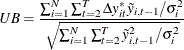
where ![]() . When
. When ![]() is unknown, it can be estimated as
is unknown, it can be estimated as
The ![]() statistic has a standard normal limiting distribution as
statistic has a standard normal limiting distribution as ![]() followed by
followed by ![]() sequentially.
sequentially.
To account for the short-run dynamics, Breitung and Das (2005) suggest applying the test to the prewhitened series, ![]() . For model (1) and model (2) (constant-only case), they suggested the same method as in step 1 of Levin, Lin, and Chu (2002).[10] For model (3) (with a constant and linear time trend), the prewhitened series can be obtained by running the following restricted
ADF regression under the null hypothesis of a unit root (
. For model (1) and model (2) (constant-only case), they suggested the same method as in step 1 of Levin, Lin, and Chu (2002).[10] For model (3) (with a constant and linear time trend), the prewhitened series can be obtained by running the following restricted
ADF regression under the null hypothesis of a unit root ( ![]() ) and no intercept and linear time trend (
) and no intercept and linear time trend (![]() ):
):
where ![]() is a consistent estimator of the true lag order
is a consistent estimator of the true lag order ![]() and can be estimated by the procedures listed in the section Lag Order Selection in the ADF Regression. For LLC and IPS tests, the lag orders are selected by running the ADF regressions. But for Breitung and his coauthors’ tests,
the restricted ADF regressions are used to be consistent with the prewhitening method. Let
and can be estimated by the procedures listed in the section Lag Order Selection in the ADF Regression. For LLC and IPS tests, the lag orders are selected by running the ADF regressions. But for Breitung and his coauthors’ tests,
the restricted ADF regressions are used to be consistent with the prewhitening method. Let ![]() be the estimated coefficients.[11] The prewhitened series can be obtained by
be the estimated coefficients.[11] The prewhitened series can be obtained by
and
The transformed series are random walks under the null hypothesis,
where ![]() for
for ![]() . When the cross-section units are independent, the t statistic converges to standard normal under the null, as
. When the cross-section units are independent, the t statistic converges to standard normal under the null, as ![]() followed by
followed by ![]() ,
,
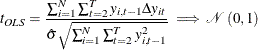
where ![]() with OLS estimator
with OLS estimator ![]() .
.
To take account for cross-sectional dependence, Breitung and Das (2005) propose the robust t statistic and a GLS version of the test statistic. Let ![]() be the error vector for time
be the error vector for time ![]() , and let
, and let ![]() be a positive definite matrix with eigenvalues
be a positive definite matrix with eigenvalues ![]() . Let
. Let ![]() and
and ![]() . The model can be written as a SUR-type system of equations,
. The model can be written as a SUR-type system of equations,
The unknown covariance matrix ![]() can be estimated by its sample counterpart,
can be estimated by its sample counterpart,
The sequential limit ![]() followed by
followed by ![]() of the standard t statistic
of the standard t statistic ![]() is normal with mean
is normal with mean ![]() and variance
and variance ![]() . The variance
. The variance ![]() can be consistently estimated by
can be consistently estimated by ![]() . Thus the robust t statistic can be calculated as
. Thus the robust t statistic can be calculated as
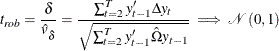
as ![]() followed by
followed by ![]() under the null hypothesis of random walk. Since the finite sample distribution can be quite different, Breitung and Das (2005) list the
under the null hypothesis of random walk. Since the finite sample distribution can be quite different, Breitung and Das (2005) list the ![]() ,
, ![]() , and
, and ![]() critical values for different
critical values for different ![]() ’s.
’s.
When ![]() , a (feasible) GLS estimator is applied; it is asymptotically more efficient than the OLS estimator. The data are transformed
by multiplying
, a (feasible) GLS estimator is applied; it is asymptotically more efficient than the OLS estimator. The data are transformed
by multiplying ![]() as defined before,
as defined before, ![]() . Thus the model is transformed into
. Thus the model is transformed into
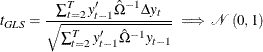
The feasible GLS (FGLS) estimator of ![]() and the corresponding t statistic are obtained by estimating the transformed model by OLS and denoted by
and the corresponding t statistic are obtained by estimating the transformed model by OLS and denoted by ![]() and
and ![]() , respectively:
, respectively:
Hadri (2000) Stationarity Tests
Hadri (2000) adopts a component representation where an individual time series is written as a sum of a deterministic trend, a random walk, and a white-noise disturbance term. Under the null hypothesis of stationary, the variance of the random walk equals 0. Specifically, two models are considered:
-
For model (1), the time series
 is stationary around a level
  ,
,

-
For model (2),
is trend stationary,

where
 is the random walk component,

The initial values of the random walks,
 , are assumed to be fixed unknowns and can be considered as heterogeneous intercepts. The errors
  and
and  satisfy
 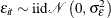 ,
,  and are mutually independent.
The null hypothesis of stationarity is ![]() against the alternative random walk hypothesis
against the alternative random walk hypothesis ![]() .
.
In matrix form, the models can be written as
where ![]() ,
, ![]() with
with ![]() , and
, and ![]() with
with ![]() being a
being a ![]() vector of ones,
vector of ones, ![]() , and
, and ![]() .
.
Let ![]() be the residuals from the regression of
be the residuals from the regression of ![]() on
on ![]() ; then the LM statistic is
; then the LM statistic is
where ![]() is the partial sum of the residuals and
is the partial sum of the residuals and ![]() is a consistent estimator of
is a consistent estimator of ![]() under the null hypothesis of stationarity. With some regularity conditions,
under the null hypothesis of stationarity. With some regularity conditions,
where ![]() is a standard Brownian bridge in model (1) and a second-level Brownian bridge in model (2). Let
is a standard Brownian bridge in model (1) and a second-level Brownian bridge in model (2). Let ![]() be a standard Wiener process (Brownian motion),
be a standard Wiener process (Brownian motion),
The mean and variance of the random variable ![]() can be calculated by using the characteristic functions,
can be calculated by using the characteristic functions,
and
The LM statistics can be standardized to obtain the standard normal limiting distribution,
Hadri’s (2000) test can be applied to the general case of heteroscedasticity and serially correlated disturbance errors. Under homoscedasticity
and serially uncorrelated errors, ![]() can be estimated as
can be estimated as
where ![]() is the number of regressors. Therefore,
is the number of regressors. Therefore, ![]() for model (1) and
for model (1) and ![]() for model (2).
for model (2).
When errors are heteroscedastic across individuals, the standard errors ![]() can be estimated by
can be estimated by ![]() for each individual
for each individual ![]() and the LM statistic needs to be modified to
and the LM statistic needs to be modified to
To allow for temporal dependence over ![]() ,
, ![]() has to be replaced by the long-run variance of
has to be replaced by the long-run variance of ![]() , which is defined as
, which is defined as ![]() . A HAC estimator can be used to consistently estimate the long-run variance
. A HAC estimator can be used to consistently estimate the long-run variance ![]() . For more information, see the section Long-Run Variance Estimation.
. For more information, see the section Long-Run Variance Estimation.
Harris and Tzavalis (1999) derive the panel unit root test under fixed ![]() and large
and large ![]() . Three models are considered as in Levin, Lin, and Chu (2002). Model (1) is the homogeneous panel,
. Three models are considered as in Levin, Lin, and Chu (2002). Model (1) is the homogeneous panel,
Under the null hypothesis, ![]() . For model (2), each series is a unit root process with a heterogeneous drift,
. For model (2), each series is a unit root process with a heterogeneous drift,
Model (3) includes heterogeneous drifts and linear time trends,
Under the null hypothesis ![]() ,
, ![]() , so the series is random walks with drift.
, so the series is random walks with drift.
Let ![]() be the OLS estimator of
be the OLS estimator of ![]() ; then
; then
where ![]() ,
, ![]() , and
, and ![]() is the projection matrix. For model (1), there are no regressors other than the lagged dependent value, so
is the projection matrix. For model (1), there are no regressors other than the lagged dependent value, so ![]() is the identity matrix
is the identity matrix ![]() . For model (2), a constant is included, so
. For model (2), a constant is included, so ![]() with
with ![]() a
a ![]() column of ones. For model (3), a constant and time trend are included. Thus
column of ones. For model (3), a constant and time trend are included. Thus ![]() , where
, where ![]() and
and ![]() .
.
When ![]() in model (1) under the null hypothesis,
in model (1) under the null hypothesis,
As ![]() , it becomes
, it becomes ![]() .
.
When the drift is absent in model (2) under the null hypothesis, ![]() ,
,
As ![]() grows large,
grows large, ![]() .
.
When the time trend is absent in model (3) under the null hypothesis, ![]() ,
,
When ![]() is sufficiently large, it implies
is sufficiently large, it implies ![]() .
.
[8] The time series length ![]() is subindexed by
is subindexed by ![]() because the panel can be unbalanced.
because the panel can be unbalanced.
[9] Choi (2001) also points out that the joint limit result where ![]() and
and ![]() go to infinity simultaneously is the same as the sequential limit, but it requires more moment conditions.
go to infinity simultaneously is the same as the sequential limit, but it requires more moment conditions.
[10] See the section Levin, Lin, and Chu (2002) for details. The only difference is the standard error estimate ![]() . Breitung suggests using
. Breitung suggests using ![]() instead of
instead of ![]() as in LLC to normalize the standard error.
as in LLC to normalize the standard error.
[11] Breitung (2000) suggests the approach in step 1 of Levin, Lin, and Chu (2002), while Breitung and Das (2005) suggest the prewhitening method as described above. In Breitung’s code, to be consistent with the papers, different approaches are adopted for model (2) and (3). Meanwhile, for the order of variable transformation and prewhitening, in model (2), the initial values are deducted (variable transformation) first, and then the prewhitening was applied. For model (3), the order is reversed. The series is prewhitened and then transformed to remove the mean and linear time trend.