The ENTROPY Procedure (Experimental)
- Overview
-
Getting Started

-
Syntax
-
DetailsGeneralized Maximum EntropyGeneralized Cross EntropyMoment Generalized Maximum EntropyMaximum Entropy-Based Seemingly Unrelated RegressionGeneralized Maximum Entropy for Multinomial Discrete Choice ModelsCensored or Truncated Dependent VariablesInformation MeasuresParameter Covariance For GCEParameter Covariance For GCE-MStatistical TestsMissing ValuesInput Data SetsOutput Data SetsODS Table NamesODS Graphics
-
Examples
- References
The ENTROPY procedure is similar in syntax to the other regression procedures in SAS. To demonstrate the similarity, suppose
the endogenous/dependent variable is y, and x1 and x2 are two exogenous/independent variables of interest. To estimate the parameters in this single equation model using PROC
ENTROPY, use the following SAS statements:
   proc entropy;
      model y = x1 x2;
   run;
Consider the following test score data compiled by Coleman et al. (1966):
title "Test Scores compiled by Coleman et al. (1966)";
data coleman;
   input test_score 6.2 teach_sal 6.2 prcnt_prof 8.2
            socio_stat 9.2 teach_score 8.2 mom_ed 7.2;
   label test_score="Average sixth grade test scores in observed district";
   label teach_sal="Average teacher salaries per student (1000s of dollars)";
   label prcnt_prof="Percent of students' fathers with professional employment";
   label socio_stat="Composite measure of socio-economic status in the district";
   label teach_score="Average verbal score for teachers";
   label mom_ed="Average level of education (years) of the students' mothers";
datalines;
37.01   3.83   28.87     7.20   26.60   6.19

   ... more lines ...
This data set contains outliers, and the condition number of the matrix of regressors, ![]() , is large, which indicates collinearity among the regressors. Since the maximum entropy estimates are both robust with respect
to the outliers and also less sensitive to a high condition number of the
, is large, which indicates collinearity among the regressors. Since the maximum entropy estimates are both robust with respect
to the outliers and also less sensitive to a high condition number of the ![]() matrix, maximum entropy estimation is a good choice for this problem.
matrix, maximum entropy estimation is a good choice for this problem.
To fit a simple linear model to this data by using PROC ENTROPY, use the following statements:
proc entropy data=coleman;
   model test_score = teach_sal prcnt_prof socio_stat teach_score mom_ed;
run;
This requests the estimation of a linear model for TEST_SCORE with the following form:
This estimation produces the “Model Summary” table in Figure 13.2, which shows the equation variables used in the estimation.
Figure 13.2: Model Summary Table
| Test Scores compiled by Coleman et al. (1966) |
| Variables(Supports(Weights)) | teach_sal prcnt_prof socio_stat teach_score mom_ed Intercept |
|---|---|
| Equations(Supports(Weights)) | test_score |
Since support points and prior weights are not specified in this example, they are not shown in the “Model Summary” table. The next four pieces of information displayed in Figure 13.3 are: the “Data Set Options,” the “Minimization Summary,” the “Final Information Measures,” and the “Observations Processed.”
Figure 13.3: Estimation Summary Tables
| Test Scores compiled by Coleman et al. (1966) |
| Data Set Options | |
|---|---|
| DATA= | WORK.COLEMAN |
| Minimization Summary | |
|---|---|
| Parameters Estimated | 6 |
| Covariance Estimator | GME |
| Entropy Type | Shannon |
| Entropy Form | Dual |
| Numerical Optimizer | Quasi Newton |
| Final Information Measures | |
|---|---|
| Objective Function Value | 9.553699 |
| Signal Entropy | 9.569484 |
| Noise Entropy | -0.01578 |
| Normed Entropy (Signal) | 0.990976 |
| Normed Entropy (Noise) | 0.999786 |
| Parameter Information Index | 0.009024 |
| Error Information Index | 0.000214 |
| Observations Processed |
|
|---|---|
| Read | 20 |
| Used | 20 |
The item labeled “Objective Function Value” is the value of the entropy estimation criterion for this estimation problem. This measure is analogous to the log-likelihood value in a maximum likelihood estimation. The “Parameter Information Index” and the “Error Information Index” are normalized entropy values that measure the proximity of the solution to the prior or target distributions.
The next table displayed is the ANOVA table, shown in Figure 13.4. This is in the same form as the ANOVA table for the MODEL procedure, since this is also a multivariate procedure.
Figure 13.4: Summary of Residual Errors
| GME Summary of Residual Errors | |||||||
|---|---|---|---|---|---|---|---|
| Equation | DF Model | DF Error | SSE | MSE | Root MSE | R-Square | Adj RSq |
| test_score | 6 | 14 | 175.8 | 8.7881 | 2.9645 | 0.7266 | 0.6290 |
The last table displayed is the “Parameter Estimates” table, shown in Figure 13.5. The difference between this parameter estimates table and the parameter estimates table produced by other regression procedures is that the standard error and the probabilities are labeled as approximate.
Figure 13.5: Parameter Estimates
| GME Variable Estimates | ||||
|---|---|---|---|---|
| Variable | Estimate | Approx Std Err | t Value | Approx Pr > |t| |
| teach_sal | 0.287979 | 0.00551 | 52.26 | <.0001 |
| prcnt_prof | 0.02266 | 0.00323 | 7.01 | <.0001 |
| socio_stat | 0.199777 | 0.0308 | 6.48 | <.0001 |
| teach_score | 0.497137 | 0.0180 | 27.61 | <.0001 |
| mom_ed | 1.644472 | 0.0921 | 17.85 | <.0001 |
| Intercept | 10.5021 | 0.3958 | 26.53 | <.0001 |
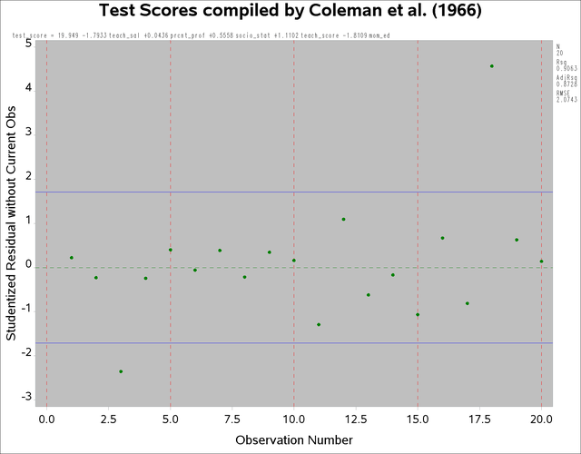
The parameter estimates produced by the REG procedure for this same model are shown in Figure 13.6. Note that the parameters and standard errors from PROC REG are much different than estimates produced by PROC ENTROPY.
symbol v=dot h=1 c=green;

proc reg data=coleman;
   model test_score = teach_sal prcnt_prof socio_stat teach_score mom_ed;
   plot rstudent.*obs.
        / vref= -1.714 1.714 cvref=blue lvref=1
          HREF=0 to 30 by 5 cHREF=red  cframe=ligr;
run;
Figure 13.6: REG Procedure Parameter Estimates
| Test Scores compiled by Coleman et al. (1966) |
| Parameter Estimates | |||||
|---|---|---|---|---|---|
| Variable | DF | Parameter Estimate |
Standard Error |
t Value | Pr > |t| |
| Intercept | 1 | 19.94857 | 13.62755 | 1.46 | 0.1653 |
| teach_sal | 1 | -1.79333 | 1.23340 | -1.45 | 0.1680 |
| prcnt_prof | 1 | 0.04360 | 0.05326 | 0.82 | 0.4267 |
| socio_stat | 1 | 0.55576 | 0.09296 | 5.98 | <.0001 |
| teach_score | 1 | 1.11017 | 0.43377 | 2.56 | 0.0227 |
| mom_ed | 1 | -1.81092 | 2.02739 | -0.89 | 0.3868 |
This data set contains two outliers, observations 3 and 18. These can be seen in a plot of the residuals shown in Figure 13.7
The presence of outliers suggests that a robust estimator such as ![]() -estimator in the ROBUSTREG procedure should be used. The following statements use the ROBUSTREG procedure to estimate the
model.
-estimator in the ROBUSTREG procedure should be used. The following statements use the ROBUSTREG procedure to estimate the
model.
proc robustreg data=coleman;
   model test_score = teach_sal prcnt_prof
                      socio_stat teach_score mom_ed;
run;
The results of the estimation are shown in Figure 13.8.
Figure 13.8: ![]() -Estimation Results
-Estimation Results
| Test Scores compiled by Coleman et al. (1966) |
| Parameter Estimates | |||||||
|---|---|---|---|---|---|---|---|
| Parameter | DF | Estimate | Standard Error | 95% Confidence Limits | Chi-Square | Pr > ChiSq | |
| Intercept | 1 | 29.3416 | 6.0381 | 17.5072 | 41.1761 | 23.61 | <.0001 |
| teach_sal | 1 | -1.6329 | 0.5465 | -2.7040 | -0.5618 | 8.93 | 0.0028 |
| prcnt_prof | 1 | 0.0823 | 0.0236 | 0.0361 | 0.1286 | 12.17 | 0.0005 |
| socio_stat | 1 | 0.6653 | 0.0412 | 0.5846 | 0.7461 | 260.95 | <.0001 |
| teach_score | 1 | 1.1744 | 0.1922 | 0.7977 | 1.5510 | 37.34 | <.0001 |
| mom_ed | 1 | -3.9706 | 0.8983 | -5.7312 | -2.2100 | 19.54 | <.0001 |
| Scale | 1 | 0.6966 | |||||
Note that TEACH_SAL(VAR1) and MOM_ED(VAR5) change greatly when the robust estimation is used. Unfortunately, these two coefficients are negative, which implies that the test scores increase with decreasing teacher salaries and decreasing levels of the mother’s education. Since ROBUSTREG is robust to outliers, they are not causing the counterintuitive parameter estimates.
The condition number of the regressor matrix ![]() also plays a important role in parameter estimation. The condition number of the matrix can be obtained by specifying the
COLLIN option in the PROC ENTROPY statement.
also plays a important role in parameter estimation. The condition number of the matrix can be obtained by specifying the
COLLIN option in the PROC ENTROPY statement.
proc entropy data=coleman collin;
   model test_score = teach_sal prcnt_prof socio_stat teach_score mom_ed;
run;
The output produced by the COLLIN option is shown in Figure 13.9.
Figure 13.9: Collinearity Diagnostics
| Test Scores compiled by Coleman et al. (1966) |
| Collinearity Diagnostics | ||||||||
|---|---|---|---|---|---|---|---|---|
| Number | Eigenvalue | Condition Number |
Proportion of Variation | |||||
| teach_sal | prcnt_prof | socio_stat | teach_score | mom_ed | Intercept | |||
| 1 | 4.978128 | 1.0000 | 0.0007 | 0.0012 | 0.0026 | 0.0001 | 0.0001 | 0.0000 |
| 2 | 0.937758 | 2.3040 | 0.0006 | 0.0028 | 0.2131 | 0.0001 | 0.0000 | 0.0001 |
| 3 | 0.066023 | 8.6833 | 0.0202 | 0.3529 | 0.6159 | 0.0011 | 0.0000 | 0.0003 |
| 4 | 0.016036 | 17.6191 | 0.7961 | 0.0317 | 0.0534 | 0.0059 | 0.0083 | 0.0099 |
| 5 | 0.001364 | 60.4112 | 0.1619 | 0.3242 | 0.0053 | 0.7987 | 0.3309 | 0.0282 |
| 6 | 0.000691 | 84.8501 | 0.0205 | 0.2874 | 0.1096 | 0.1942 | 0.6607 | 0.9614 |
The condition number of the ![]() matrix is reported to be
matrix is reported to be ![]() . This means that the condition number of
. This means that the condition number of ![]() is
is ![]() , which is very large.
, which is very large.
Ridge regression can be used to offset some of the problems associated with ill-conditioned ![]() matrices. Using the formula for the ridge value as
matrices. Using the formula for the ridge value as
where ![]() and
and ![]() are the least squares estimators of
are the least squares estimators of ![]() and
and ![]() and
and ![]() . A ridge regression of the test score model was performed by using the data set with the outliers removed. The following
PROC REG code performs the ridge regression:
. A ridge regression of the test score model was performed by using the data set with the outliers removed. The following
PROC REG code performs the ridge regression:
data coleman;
   set coleman;
   if _n_ = 3 or _n_ = 18 then delete;
run;
proc reg data=coleman ridge=0.9 outest=t noprint;
   model test_score = teach_sal prcnt_prof socio_stat teach_score mom_ed;
run;

proc print data=t;
run;
The results of the estimation are shown in Figure 13.10.
Figure 13.10: Ridge Regression Estimates
| Test Scores compiled by Coleman et al. (1966) |
| Obs | _MODEL_ | _TYPE_ | _DEPVAR_ | _RIDGE_ | _PCOMIT_ | _RMSE_ | Intercept | teach_sal | prcnt_prof | socio_stat | teach_score | mom_ed | test_score |
|---|---|---|---|---|---|---|---|---|---|---|---|---|---|
| 1 | MODEL1 | PARMS | test_score | . | . | 0.78236 | 29.7577 | -1.69854 | 0.085118 | 0.66617 | 1.18400 | -4.06675 | -1 |
| 2 | MODEL1 | RIDGE | test_score | 0.9 | . | 3.19679 | 9.6698 | -0.08892 | 0.041889 | 0.23223 | 0.60041 | 1.32168 | -1 |
Note that the ridge regression estimates are much closer to the estimates produced by the ENTROPY procedure that uses the original data set. Ridge regressions are not robust to outliers as maximum entropy estimates are. This might explain why the estimates still differ for TEACH_SAL.