The COPULA Procedure
- Overview
- Getting Started
-
Syntax

-
DetailsSklar’s TheoremDependence MeasuresNormal CopulaStudent’s t copulaArchimedean CopulasCanonical Maximum Likelihood Estimation (CMLE)Exact Maximum Likelihood Estimation (MLE)Calibration EstimationNonlinear Optimization OptionsDisplayed OutputOUTCOPULA= Data SetOUTPSEUDO=, OUT=, and OUTUNIFORM= Data SetsODS Table NamesODS Graph Names
-
Examples
- References
Let ![]() for
for ![]() , where
, where ![]() represents the uniform distribution on the
represents the uniform distribution on the ![]() interval. Let
interval. Let ![]() be the correlation matrix with
be the correlation matrix with ![]() parameters satisfying the positive semidefiniteness constraint. The normal copula can be written as
parameters satisfying the positive semidefiniteness constraint. The normal copula can be written as
where ![]() is the distribution function of a standard normal random variable and
is the distribution function of a standard normal random variable and ![]() is the
is the ![]() -variate standard normal distribution with mean vector
-variate standard normal distribution with mean vector ![]() and covariance matrix
and covariance matrix ![]() . That is, the distribution
. That is, the distribution ![]() is
is ![]() .
.
For the normal copula, the input of the simulation is the correlation matrix ![]() . The normal copula can be simulated by the following steps in which
. The normal copula can be simulated by the following steps in which ![]() denotes one random draw from the copula:
denotes one random draw from the copula:
-
Generate a multivariate normal vector
 where
where  is an
is an  -dimensional correlation matrix.
-
Transform the vector
 into
into 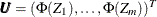 , where
  is the distribution function of univariate standard normal.
The first step can be achieved by Cholesky decomposition of the correlation matrix ![]() where
where ![]() is a lower triangular matrix with positive elements on the diagonal. If
is a lower triangular matrix with positive elements on the diagonal. If ![]() , then
, then ![]() .
.
To fit a normal copula is to estimate the covariance matrix ![]() from an input sample data set. Given a random sample
from an input sample data set. Given a random sample ![]() where
where ![]() , the log-likelihood function is
, the log-likelihood function is
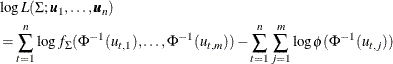
Here ![]() is the joint density of the multivariate normal with mean zero and variance
is the joint density of the multivariate normal with mean zero and variance ![]() , and
, and ![]() is the univariate density of the standard normal distribution. Note that the second term is not related to the parameters
is the univariate density of the standard normal distribution. Note that the second term is not related to the parameters
![]() and, therefore, can be ignored during the optimization. The restriction that
and, therefore, can be ignored during the optimization. The restriction that ![]() is a correlation matrix is very inconvenient, and it is common practice to circumvent this problem by first assuming that
is a correlation matrix is very inconvenient, and it is common practice to circumvent this problem by first assuming that
![]() has the covariance form. Therefore,
has the covariance form. Therefore, ![]() can be estimated by
can be estimated by
where
This estimate is consistent with the form of a covariance matrix but not necessarily with the form of a correlation matrix. The approximation to the original MLE problem can be obtained using the normalizing operator defined as follows: